9 Continuous RVs: Uniform & Normal

NEW NOTATION:

\(\propto\) = “proportional to”

\(y = 5x^2\) \(\;\; \Rightarrow \;\;\) \(y \propto x^2\)

\(y\) = height in inches, \(x\) = height in centimeters
\(y = 2.54x\) \(\;\; \Rightarrow \;\;\) \(y \propto x\)

there’s a constant ratio between \(y\) and \(x\)
\(y \propto x\)

READING:

For more on this topic, read B & H Chapter 5.1 - 5.2.

9.1 Discussion

EXAMPLE 1

Let \(X\) be the speed of a car on highway 94. Draw a reasonable model for \(X\).

Probability Models for Continuous RVs

Let \(X\) be a continuous RV. A probability density function (pdf) \(f_X(x)\) describes the plausible values of \(X\) and their relative likelihoods. A valid pdf satisfies

\(f_X(x) \ge 0\)

\(\int_{-\infty}^{\infty} f_X(x) dx = 1\)

Detail: \(X\) vs \(x\)

\(X\) is a label for the random variable. \(x\) is the value of \(X\) that we observe.

EXAMPLE 2

Let \(Y\) be the proportion of 1 MN winter day that has significant cloud cover. Suppose \(Y\) has pdf \[f_Y(y) \propto 1-y \;\; \text{ for } y \in [0,1]\] That is, for some normalizing constant \(c\), \[f_Y(y) = c(1-y) \;\; \text{ for } y \in [0,1]\]

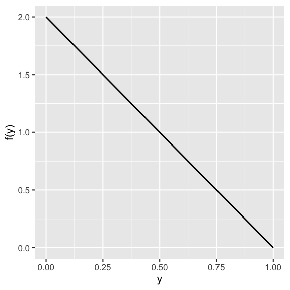
Determine the value of the normalizing constant \(c\) that makes \(f_Y(y)\) a valid pdf.
Calculate the probability that more than 50% of the day has cloud cover.
Calculate the probability that exactly 50% of the day has cloud cover.

Using & interpreting pdfs

\(P(X \in (a,b)) = \int_a^b f_X(x)dx\)

\(P(X = a) = \int_a^a f_X(x)dx = 0\)

We cannot interpret the pdf as a probability. In fact, \(f_X(x)\) can be >1. Plus the probability of any given value is 0!

Named probability models

In the exercises below, you’ll build up and study two of the most famous continuous probability models, the Uniform and Normal. The Uniform is a good model when RV \(X\) is uniformly or equally likely to take on any value in a given range:

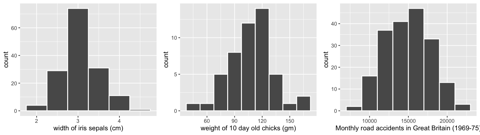
The Normal (aka “Gaussian”) model is so named because its patterns are so commonly observed in data. Just a few examples:

History of the Normal (Gaussian) model

Abraham De Moivre (∼ 1733)
“Discovered” the Normal model while trying to approximate the large binomial coefficients in Pascal’s triangle. His motivation? Gambling and actuarial tables.
Carl Friedrich Gauss (∼ 1795)
While studying planetary motion, noticed that the errors in astronomical measurements have a Normal model.
Pierre-Simon de Laplace (∼ 1810)
Came across Gauss’ results in 1810, slipped into the end of a book. He plucked it from obscurity.
Adolphe Quetelet (∼ 1835)
“Discovered” that the Normal model could also be applied to social data: physical characteristics, crime, mortality (by age, geography, season, profession, etc), drunkenness, insanity, marriage, etc. Quetelet observed a nice, Normal model everywhere! Except 1 place: the heights of 100,000 French men called up for the army draft. Guess why before peaking at the answer.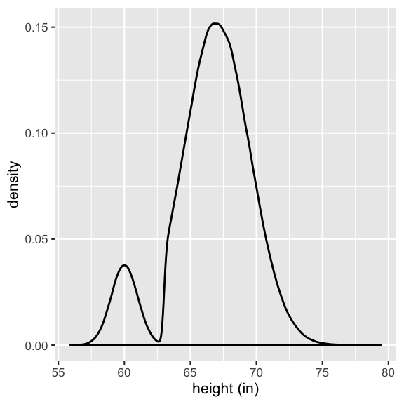

Models vs reality

George Box said that “All models are wrong. Some models are useful.” For example, note that the Normal model is technically defined on \((-\infty,\infty)\). However, it’s a useful approximation of RVs that have restricted support. For example, human heights can’t be negative, but are still well-approximated by a Normal. Similarly, SAT scores are both discrete and limited to a specific range, but are still well-approximated by a Normal.

9.2 Exercises

9.2.1 Uniform

Case 1: Unif(0,6)
You use a computer random number generator to pick a number, \(U\), that’s equally likely to be anywhere between 0 and 6.
1. Specify a formula for and sketch the pdf \(f_U(u)\). HINT: Remember that \(f_U(u)\) must integrate to 1!
2. Calculate the following probabilities & represent these in your sketch:
  - \(P(U \ge 5)\)
  - \(P(U > 5)\)
  - \(P(U = 5)\)

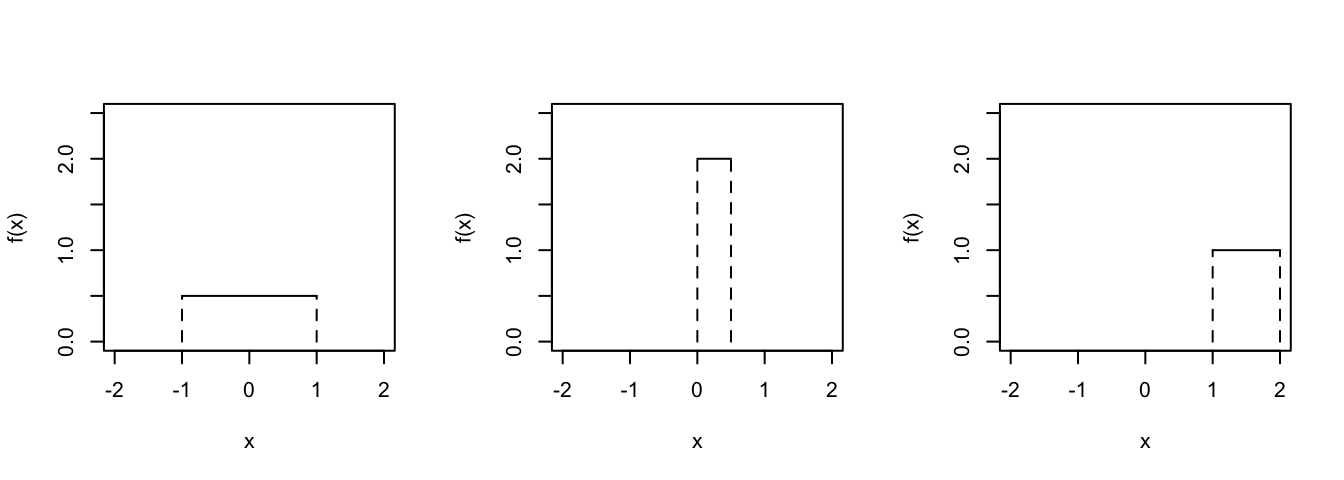
Case 2: Unif(0,0.5)
Similarly, use a computer random number generator to pick a number, \(V\), that’s equally likely to be anywhere between 0 and 0.5.
1. Specify a formula for and sketch the pdf \(f_V(v)\).
2. Is it a problem that \(f_V(v) > 1\)?!
3. Identify the 25th percentile, or 0.25 quantile of \(V\). That is, identify the value of \(v\) for which \[P(V \le v) = 0.25\]

The continuous Uniform model
In general, suppose random variable \(X\) is equally / uniformly distributed across the interval \([a, b]\). In notation, \[X \sim Unif(a, b)\] where \(a\) and \(b\) are model parameters.
1. Specify and sketch the pdf of \(X\), \(f_X(x)\), in this general setting.
2. Provide a general formula for calculating \(P(X \le x)\) for some \(x \in [a,b]\).

9.2.2 Normal

A Normal RV is specified by 2 parameters, \(\mu\) and \(\sigma\):

\[X \sim N(\mu, \sigma^2)\]

and has pdf

\[f_X(x) = \frac{1}{\sqrt{2 \pi \sigma^2}} e^{-\frac{1}{2}\left(\frac{x-\mu}{\sigma} \right)^2} = \frac{1}{\sqrt{2 \pi \sigma^2}} \exp\left\lbrace -\frac{1}{2}\left(\frac{x-\mu}{\sigma} \right)^2\right\rbrace \;\;\; \text{ for } x \in (-\infty,\infty)\]

Normal properties
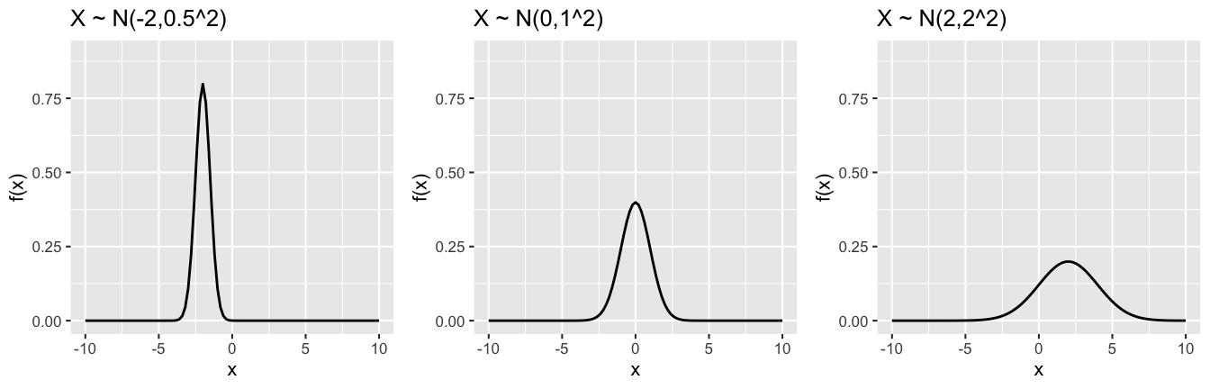
The pdfs of 3 different Normal models are plotted below. All 3 Normal models have a bell shape. Explain how the \(\mu\) and \(\sigma\) parameters inform this shape.

The Standard Normal Model
The special case of a Normal RV with mean 0 & variance 1 is referred to as the standard Normal: \[Z \sim N(0,1^2)\]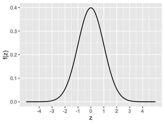
1. Specify the formula for the pdf of \(Z\), \(f(z)\).
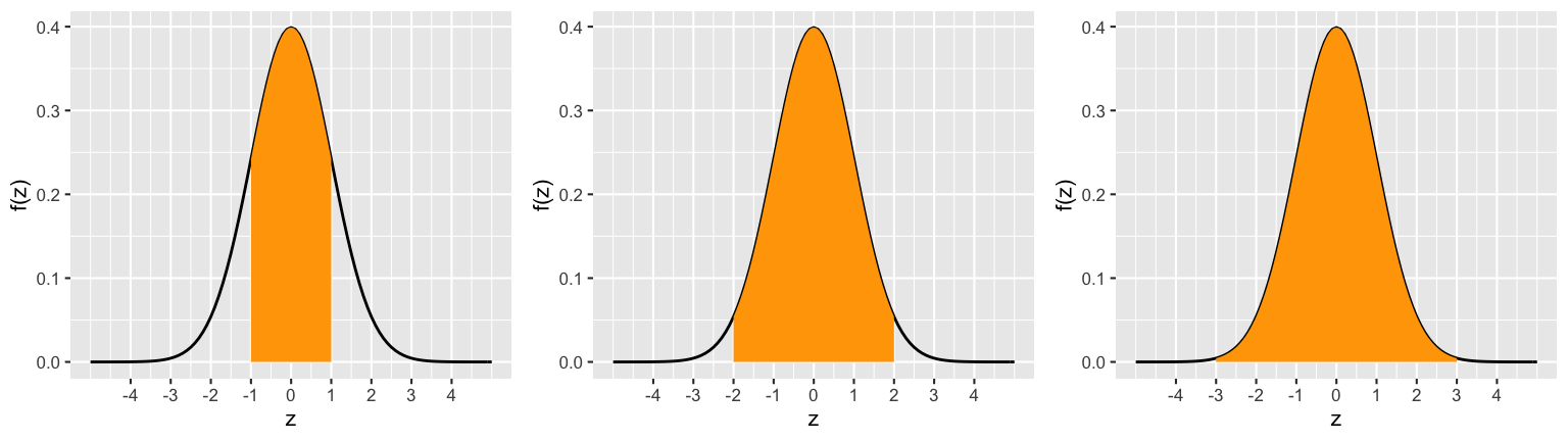
2. Utilize the output below to calculate the probability that \(Z\) is within 1 unit of 0, \(P(-1 < Z < 1)\). Sketching a picture would help!
```
# Probability Z is BELOW 1
pnorm(1, 0, 1)
## [1] 0.8413447

# Probability Z is BELOW -1
pnorm(-1, 0, 1)
## [1] 0.1586553
```
3. Calculate the probability that \(Z\) is within 2 units of 0, \(P(-2 < Z < 2)\).
```
pnorm(2, 0, 1)
## [1] 0.9772499
pnorm(-2, 0, 1)
## [1] 0.02275013
```
4. Calculate the probability that \(Z\) is within 3 units of 0, \(P(-3 < Z < 3)\).
```
pnorm(3, 0, 1)
## [1] 0.9986501
pnorm(-3, 0, 1)
## [1] 0.001349898
```
In pictures:

68-95-99.7 Rule
In the exercise above, you established the “68-95-99.7 Rule” for the standard Normal RV \(Z \sim N(0,1^2)\). This rule extends to all \(X \sim N(\mu, \sigma^2)\) models:
- 68% of \(X\) values are within 1 \(\sigma\) of \(\mu\)
- 95% of \(X\) values are within 2 \(\sigma\) of \(\mu\)
- 99.7% of \(X\) values are within 3 \(\sigma\) of \(\mu\)
In notation:

\[\begin{split} P(\mu - \sigma < X < \mu + \sigma) & = \int_{\mu - \sigma}^{\mu + \sigma} f_X(x)dx \approx 0.68 \\ P(\mu - 2\sigma < X < \mu + 2\sigma) & = \int_{\mu - 2\sigma}^{\mu + 2\sigma} f_X(x)dx \approx 0.95 \\ P(\mu - 3\sigma < X < \mu + 3\sigma) & = \int_{\mu - 3\sigma}^{\mu + 3\sigma} f_X(x)dx \approx 0.997 \\ \end{split}\]
Why do we care?! This rule gives us a sense of how to interpret the scale of the \(\sigma\). It’s also utilized in statistical hypothesis testing (which we’ll touch on toward the end of the semester).
1. To convince yourself this is true, establish this property for \(X \sim N(110, 20^2)\), the weight in grams of 10 day old chicks.
2. Suppose the instructor tells you that students’ grades on the midterm can be modeled by \(X \sim N(80, 5^2)\). What does this tell you about the typical range of exam scores?

9.2.3 Optional: Normal vs Poisson vs Binomial

NOTE: These exercises are on Homework 4!

We’ve been discussing a growing collection of special models. Each of these has unique features with unique applications in unique settings. However, there are also similarities among these models in certain settings. For example, notice the similarities among the Binomial, Poisson, and Normal RVs plotted below:

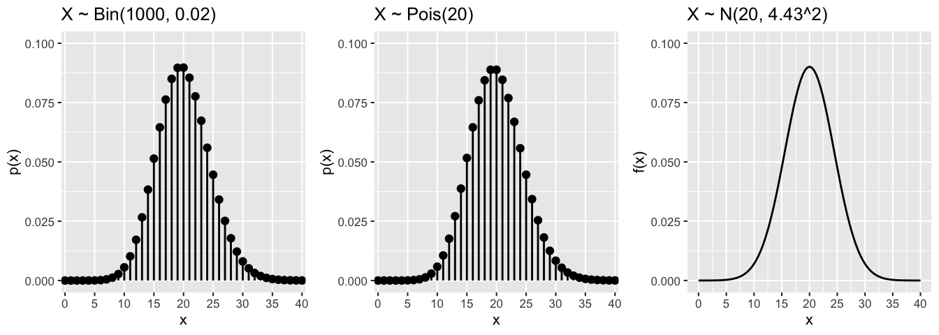
When Binomial \(\approx\) Normal \(\approx\) Poisson
1. In the example above, the \(Bin(n,p)\) model had large \(n\) (1000) and small \(p\) (0.02). Provide an intuitive explanation why in the large \(n\) and small \(p\) scenario, the \(Bin(n,p)\) model is approximately \(Pois(np)\). (You’ll prove this below.)
2. Similarly, provide an intuitive explanation why in the large \(n\) scenario, the \(Bin(n,p)\) model is approximately \(N(np, np(1-p))\). (We won’t have the tools to prove this until the end of the semester.)
3. Let’s prove that if \(X \sim Bin(n,p)\) and we let \(n \to \infty\) and \(p \to 0\) so that \(\lambda = np\) remains fixed, then \(X\) is approximately \(Pois(\lambda)\). You can do this in two steps:
  - Step 1
    Prove that we can rewrite the pmf of \(X\) as \[p_X(x) = \left(\begin{array}{c} n \\ x \end{array} \right) p^x (1-p)^{n-x} = \frac{\lambda^x}{x!} \frac{n(n-1)\cdots (n-x+1)}{n^x} \left(1 - \frac{\lambda}{n}\right)^n\left(1 - \frac{\lambda}{n} \right)^{-x}\]
  - Step 2
    Prove that as \(n \to \infty\) and \(p \to 0\) (so that \(\lambda = np\) remains fixed), the Binomial pmf converges to the Poisson pmf: \[p_X(x) \to \frac{e^{-np}(np)^x}{x!}\] That is, \[X \sim Bin(n,p) \to X \sim Pois(np)\]
    
    HINT: \(\left(1 - \frac{\lambda}{n}\right)^n \to e^{-\lambda}\).