15 Dusting off

Goals

Review:

random variables (RVs)
univariate models
RV transformations

15.1 Review: RVs

A random variable $X$ is a function from the sample space $S$ to the real line $\mathbb{R}$. That is, $X$ is a numerical outcome of an experiment.

EXAMPLE

$X$ is a baby’s birth weight (in pounds). A probability model of $X$ describes:

possible values of $X$
relative plausibility of these values

A reasonable probability model for $X$ is

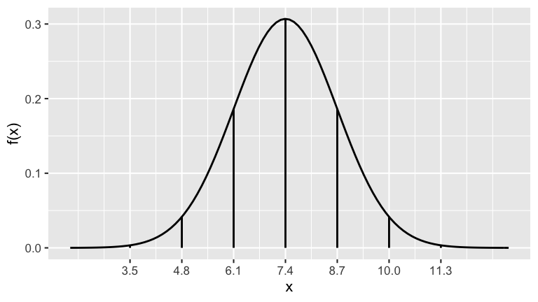
\[X \sim N(7.4, 1.3^2)\]

Properties

probability density function (pdf) \[f(x) = \frac{1}{\sqrt{2\pi \cdot 1.3^2}} e^{-\frac{1}{2}\left(\frac{x - 7.4}{1.3} \right)^2}\;\; \text{ for } x \in (-\infty, \infty)\]
cumulative distribution function (cdf)
\[F(t) = P(X \le t) = \int_{-\infty}^tf(x)dx\]
$E(X) = 7.4$ pounds
$Var(X) = 1.3^2$ pounds$^2$
$SD(X) = 1.3$ pounds

Our current collection of named probability models

model	common application	$E(X)$	$Var(X)$
Bin($n,p$)	# of successes in $n$ trials	$np$	$np(1-p)$
Geo($p$)	# of trials until 1st success	$\frac{1}{p}$	$\frac{1-p}{p^2}$
Pois($\lambda$)	# of events in a given time interval	$\lambda$	$\lambda$
N($\mu,\sigma^2$)	RVs with bell-shaped distributions	$\mu$	$\sigma^2$
Exp($\lambda$)	continuous waiting time for 1 event	$\frac{1}{\lambda}$	$\frac{1}{\lambda^2}$
Gamma($a,\lambda$)	continuous waiting time for $a$ events	$\frac{a}{\lambda}$	$\frac{a}{\lambda^2}$

15.2 Review: Functions of RVs

For RV $X$ (discrete or continuous), let $Y$ be a linear transformation of $X$:

\[Y = aX + b \;\; \text{ for } a,b \in \mathbb{R}\]

Such transformations are common. For example:

$X$ = temperature in Fahrenheit
$Y = \frac{5}{9}(X-32)$ = temperature in Celsius
$X$ = height in centimeters
$Y = 2.54 X$ = height in inches

Examples

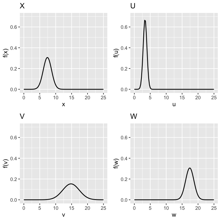
Let $X$ be baby birth weight in pounds:

\[X \sim N(7.4, 1.3^2)\]

Consider 3 transformations of $X$:

\[\begin{split} U & = 0.454 X \text{ (birth weight in kg)}\\ V & = 2X \\ W & = X + 10 \\ \end{split}\]

Properties of $Y$

Let $Y = aX + b$. Then we can obtain the properties of $Y$ from the properties of $X$:

\[\begin{split} E(Y) & = a E(X) + b \\ Var(Y) & = a^2 Var(X) \\ \end{split}\]

Further,

\[\begin{split} X \text{ discrete } \Rightarrow \;\; & p_Y(y) = p_X\left(\frac{y - b}{a} \right) \\ X \text{ continuous } \Rightarrow \;\; & f_Y(y) = \frac{1}{|a|}f_X\left(\frac{y - b}{a} \right) \\ \end{split}\]

Interpretation

$a$ = a change in scale and $b$ = a change in location
The expected value of a RV is impacted by both a change in location ($b$) and scale ($a$)
The variance of a RV isn’t impacted by a change in location ($b$) but is impacted by a change in scale ($a$).

Proof

Assume $X$ is continuous. The proof for discrete $X$ is similar.

\[\begin{split} E(Y) & = E(aX + b) \\ & = \int (ax+b)f_X(x)dx \\ & = \int (axf_X(x) + bf_X(x))dx \\ & = a\int xf_X(x)dx + b\int f_X(x)dx \\ & = aE(X) + b \\ & \\ Var(Y) & = Var(aX + b) \\ & = E((aX+b - E(aX+b))^2) \\ & = E((aX - aE(X)))^2) \\ & = E(a^2(X - E(X))^2) \\ & = a^2 E((X - E(X))^2) \;\;\;\; \text{ (we've seen we can take constants out of E()} \\ & = a^2 Var(X) \\ & \\ \text{ when } a > 0: & \\ F_Y(y) & = P(Y \le y) \\ & = P(aX+b \le y) \\ & = P(X \le (y-b)/a) \\ & = F_X((y-b)/a) \\ f_Y(y) & = F'_Y(y) = \frac{1}{a}f_X((y-b)/a) \\ & \\ \text{ when } a < 0: & \\ F_Y(y) & = P(Y \le y) \\ & = P(aX+b \le y) \\ & = P(X \ge (y-b)/a) \\ & = 1 - P(X \le (y-b)/a) \\ & = 1 - F_X((y-b)/a) \\ f_Y(y) & = F'_Y(y) = \frac{1}{-a}f_X((y-b)/a) = \frac{1}{|a|}f_X((y-b)/a) \\ \end{split}\]

LINEAR TRANSFORMATION OF THE NORMAL

Let $X \sim N(\mu,\sigma^2)$ with

\[\begin{split} f_X(x) & = \frac{1}{\sqrt{2 \pi \sigma^2}} e^{-\frac{1}{2}\left(\frac{x - \mu}{\sigma}\right)^2} \;\;\; \text{ for } x \in (-\infty,\infty) \\ E(X) & = \mu \\ Var(X) & = \sigma^2 \\ \end{split}\]

Let

\[Y = \frac{X - \mu}{\sigma} = \frac{1}{\sigma} X - \frac{\mu}{\sigma}\]

Show that:

$E(Y) = 0$
$SD(Y) = 1$
$Y \sim N(0, 1^2)$, ie. $Y$ is standard normal.

NOTE: Similarly, if $Y \sim N(0,1)$ and $X = \sigma Y +\mu$, we could show that $X \sim N(\mu,\sigma^2)$!

PROOF:

Since $Y = \frac{X - \mu}{\sigma} = \frac{1}{\sigma}X - \frac{\mu}{\sigma}$, $Y = aX + b$ where $a = 1/\sigma$ and $b = -\mu/\sigma$. Thus

\[\begin{split} f_Y(y) & = \frac{1}{a}f_X\left(\frac{y -b}{a} \right) \\ & = \frac{1}{1/\sigma}f_X\left(\frac{y + \mu/\sigma}{1/\sigma} \right) \\ & = \sigma f_X\left(\sigma y + \mu \right) \\ & = \frac{\sigma}{\sqrt{2 \pi \sigma^2}} \exp\left\lbrace -\frac{1}{2}\left(\frac{(\sigma y + \mu) -\mu}{\sigma} \right)^2\right\rbrace \\ & = \frac{1}{\sqrt{2 \pi}} \exp\left\lbrace -\frac{1}{2}y^2\right\rbrace \;\;\; \text{ for } y \in (-\infty,\infty) \\ \end{split}\] which is the pdf of $N(0,1^2)$. Further,

\[\begin{split} E(Y) & = \frac{1}{\sigma}E(X) - \frac{\mu}{\sigma} = \frac{1}{\sigma}\mu - \frac{\mu}{\sigma} = 0 \\ Var(Y) & = \frac{1}{\sigma^2} Var(X) = \frac{1}{\sigma^2} \sigma^2 = 1 \\ \end{split}\]

EXAMPLE: What’s the point?

Let $X$ be baby birth weight:

\[X \sim N(7.4, 1.3^2)\]

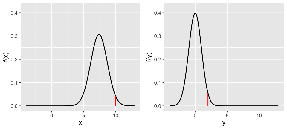
And $Y$ be the standardized value of $X$:

\[Y = \frac{X - 7.4}{1.3} = \text{ the number of s.d. that $X$ is from 7.4}\]

For example, suppose a baby weighs $X = 10$ pounds. Then their birth weight is 2 standard deviations above the mean:

\[Y = \frac{10 - 7.4}{1.3} = 2\]

model	common application	\(E(X)\)	\(Var(X)\)
Bin(\(n,p\))	# of successes in \(n\) trials	\(np\)	\(np(1-p)\)
Geo(\(p\))	# of trials until 1st success	\(\frac{1}{p}\)	\(\frac{1-p}{p^2}\)
Pois(\(\lambda\))	# of events in a given time interval	\(\lambda\)	\(\lambda\)
N(\(\mu,\sigma^2\))	RVs with bell-shaped distributions	\(\mu\)	\(\sigma^2\)
Exp(\(\lambda\))	continuous waiting time for 1 event	\(\frac{1}{\lambda}\)	\(\frac{1}{\lambda^2}\)
Gamma(\(a,\lambda\))	continuous waiting time for \(a\) events	\(\frac{a}{\lambda}\)	\(\frac{a}{\lambda^2}\)