12 PAUSE: Random Variables in Practice

Thus far in Unit 2:

Under the overarching goal of exploring univariate probability models, we have questioned:

What model is appropriate for any given random variable? Tools: pmf, pdf, cdf, named probability models (Uniform, Normal, Poisson, Binomial)
What are the features of a given model? Tools: expected value, variance, cdf

Thus far, we’ve focused on theoretical models and their features. In this activity, you’ll explore the behavior of data generated from these models.

Getting started

# Load packages
library(ggplot2)
library(dplyr)

Directions

Open the Rmd template provided on Moodle. Once you get a chunk working without error, be sure to remove the eval = FALSE from that chunk.
The probability concepts are the most important part of this activity. The simulation / R code merely support our exploration of these concepts. With this in mind, pay careful attention along the way and keep track of the emerging patterns. You’ll be asked to summarize these at the end of the activity.

12.1 Part 1: Normal simulation

Let \(X\) measure body temperature in degrees Celsius and suppose that a reasonable model of \(X\) is \[X \sim N(37, (5/12)^2)\] with \(E(X) = 37\) degrees and \(SD(X) = 5/12\) degrees. Simulate a sample of body temperatures for 10000 individuals. How closely do the sample features follow the properties of the underlying theoretical model?

# Simulate data
body_temps <- data.frame(x = rnorm(10000, mean = 37, sd = 5/12))

# Numerical summaries
body_temps %>% 
  summarize(mean(x), sd(x), var(x))
##    mean(x)     sd(x)    var(x)
## 1 37.00847 0.4185848 0.1752132

# Visual summary
ggplot(body_temps, aes(x = x)) + 
  geom_density()

# Sample ("empirical") cdf
ggplot(body_temps, aes(x = x)) + 
  stat_ecdf()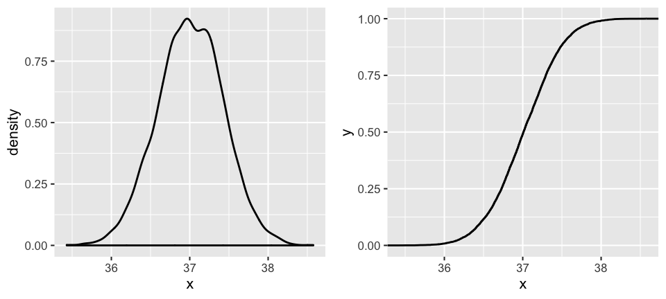

U = X + b
Define a new variable \(U = X + 32\), which adds 32 degrees to body temperatures \(X\).
1. Gut check: On a scratch piece of paper, sketch what you imagine the probability model / pdf of \(U\) will look like. Think: How, if at all, does adding 32 change the expected value, variance, or shape of the model?
2. Check your intuition. Transform your sample of \(X\) values into a sample of \(U\) values:
```
body_temps <- body_temps %>% 
  mutate(u = x + 32)
```
  Construct visual and numerical summaries of your \(U\) sample values. Was your intuition correct?
```
# Numerical summaries
body_temps %>% 
  ___(___, ___, ___)

# Visual summary
ggplot(body_temps, aes(___)) + 
  ___()
```

V = aX
Define another new variable \(V = \frac{9}{5}X\), which scales body temperatures \(X\) by 9/5.
1. Gut check: On a scratch piece of paper, sketch what you imagine the probability model / pdf of \(V\) will look like. Think: How, if at all, does scaling \(X\) by 9/5 change the expected value, variance, or shape of the model?
2. Check your intuition. Transform your sample of \(X\) values into a sample of \(V\) values:
```
body_temps <- body_temps %>% 
  mutate(v = 9/5*x)
```
  Construct visual and numerical summaries of your \(V\) sample values. Was your intuition correct?
```
# Numerical summaries
body_temps %>% 
  ___(___, ___, ___)

# Visual summary
ggplot(body_temps, aes(___)) + 
  ___()
```

Y = aX + b
Finally, define variable \(Y = \frac{9}{5}X + 32\). This transformation of \(X\) converts body temperatures from Celsius to Fahrenheit!
1. Gut check: On a scratch piece of paper, sketch what you imagine the probability model / pdf of \(Y\) will look like.
2. Check your intuition. Transform your sample of \(X\) values into a sample of \(Y\) values. Then construct visual and numerical summaries of your \(Y\) sample values. For comparison, plot \(Y\) relative to \(X\):
```
# Define y
body_temps <- ___ %>% 
  ___(y = ___)

# Numerical summaries
body_temps %>% 
  ___(___, ___, ___)

# Visual summary
ggplot(body_temps, aes(x = x)) + 
  geom_density() + 
  geom_density(aes(x = y), color = "red")
```

12.2 Part 2: Uniform simulation

Let \(X \sim \text{Unif}(0,1)\) with \(E(X) = 1/2\), \(Var(X) = 1/12\), and pdf

\[\begin{split} f_X(x) & = 1 \;\; \text{ for } x \in [0,1] \\ \end{split}\]

Simulate and examine a sample of 10000 \(X\) values:

# Simulate data
unif_sim <- data.frame(x = runif(10000, min = 0, max = 1))

# Numerical summaries
unif_sim %>% 
  summarize(mean(x), sd(x), var(x))
##     mean(x)     sd(x)     var(x)
## 1 0.4985787 0.2874904 0.08265076

# Visual summary
ggplot(unif_sim, aes(x = x)) + 
  geom_density()

# Sample ("empirical") cdf
ggplot(unif_sim, aes(x = x)) + 
  stat_ecdf()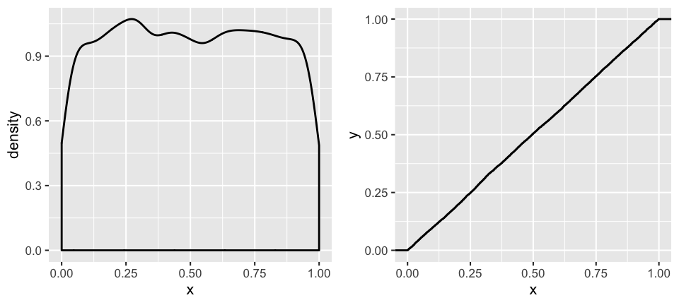

Transforming the Uniform
Let \(U\), \(V\), and \(Y\) be the following transformations of \(X\):

\[\begin{split} U & = 2X + 1 \;\;\; \text{(a linear transformation)}\\ V & = 0.5X - 1 \;\;\; \text{(a linear transformation)}\\ Y & = X^2 \;\;\; \text{(a NONlinear transformation)} \\ \end{split}\]

Gut check: On a scratch piece of paper, sketch what you imagine the probability models / pdfs of \(U\), \(V\), and \(Y\) to look like.

Check your intuition. Transform your sample of \(X\) values into a samples of \(U,V,Y\) values. Then construct visual and numerical summaries of \(U,V,Y\) sample values.

# Define u, v, y
unif_sim <- unif_sim %>% 
  ___(u = ___, v = ___, y = ___)

# Numerical summaries
unif_sim %>% 
  ___(___, ___, ___)

# Visual summary (use the same axis scales for comparison)
ggplot(unif_sim, aes(x = x)) + 
  geom_density() + 
  lims(x = c(-1, 3), y = c((0, 2.5)))
ggplot(unif_sim, aes(x = u)) + 
  geom_density() + 
  lims(x = c(-1, 3), y = c((0, 2.5)))
ggplot(unif_sim, aes(x = v)) + 
  geom_density() + 
  lims(x = c(-1, 3), y = c((0, 2.5)))
ggplot(unif_sim, aes(x = y)) + 
  geom_density() + 
  lims(x = c(-1, 3), y = c((0, 2.5)))

Do \(U\) and \(V\) look Uniform? What about \(Y\)?

12.3 Part 3: Binomial simulation

Let \(X \sim \text{Bin}(10,0.5)\) with \(E(X) = 5\) and \(Var(X) = 2.5\). Simulate and examine a sample of 10000 \(X\) values:

# Simulate data
binom_sim <- data.frame(x = rbinom(10000, size = 10, prob = 0.5))

# Numerical summaries
binom_sim %>% 
  summarize(mean(x), sd(x), var(x))
##   mean(x)    sd(x)   var(x)
## 1    4.99 1.557736 2.426543

# Visual summary
ggplot(binom_sim, aes(x = x)) + 
  stat_count()

# Sample ("empirical") cdf
ggplot(binom_sim, aes(x = x)) + 
  stat_ecdf()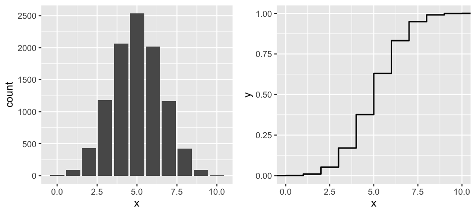

Linear transformations
Let \(Y\) be the following linear transformation of \(X\): \[Y = 0.5 X\]
1. Gut check: On a scratch piece of paper, sketch what you imagine the probability model / pmf of \(Y\) to look like.
2. Check your intuition. Transform your sample of \(X\) values into a sample of \(Y\) values. Then construct visual and numerical summaries of your \(Y\) sample values.
```
# Define y
binom_sim <- binom_sim %>% 
  ___(y = ___)

# Numerical summaries
binom_sim %>%
  ___(___, ___, ___)

# Visual summary
ggplot(binom_sim, aes(x = ___)) + 
  stat_count()
```
3. Does \(Y\) look Binomial?

12.4 Part 4: Bringing it together

You experienced above that a function of a random variable is itself a random variable with different properties! After reflecting on your simulations, try to summarize the general properties that emerged along the way.

Linear transformations: general properties
Let \(X\) be any random variable and \(Y\) be a linear transformation of \(X\):

\[Y = aX + b\]
1. Will the probability model of \(Y\) necessarily be from the same family as the probability model of \(X\)? For example:
  - If \(X\) is Normal will \(Y\) be Normal?
  - If \(X\) is Uniform will \(Y\) be Uniform?
  - If \(X\) is Binomial will \(Y\) be Binomial?
2. In words: How (if at all) does \(b\) impact the expected value? How (if at all) does \(b\) impact the variance?
3. In words: How (if at all) does \(a\) impact the expected value? How (if at all) does \(a\) impact the variance?

Linear transformations: theoretical properties
Suppose \(X\) is continuous with pdf \(f_X(x)\), \(E(X)\), and \(Var(X)\). (The proof for discrete random variables is similar.)
1. Based on your simulations above, how do you think we can write \(E(Y)\) in terms of \(E(X)\), \(a\), and \(b\)? \[E(Y) = ???\]
2. Challenge: provide a proof of your answer to part a.
3. Based on your simulations above, how do you think we can write \(Var(Y)\) in terms of \(Var(X)\), \(a\), and \(b\)? \[Var(Y) = ???\]
4. Challenge: provide a proof of your answer to part c.

BONUS challenge
The expected value and variance, \(E(Y)\) and \(Var(Y)\), provide key features of \(Y\). But what can we say about overall model of \(Y\)?
1. Assume \(X\) is discrete with pmf \(p_X(x)\). Construct the pmf of \(Y\), \(p_Y(y)\).
2. Assume \(X\) is continuous with pdf \(f_X(x)\). Construct the pdf of \(Y\), \(f_Y(y)\). HINT: First derive \(F_Y()\) from \(F_X()\), then \(f_Y()\) from \(F_Y()\).