18 Discrete: joint & conditional models

READING

For more on this topic, read B & H Chapter 7.1 - 7.2.

18.1 Discussion

EXAMPLE 1: marginal models

Roll a die six times. Let

\[\begin{split} X & = \text{ # of 4's in the 6 rolls} \\ Y & = \text{ # of 4's in the first 2 rolls} \\ \end{split}\]

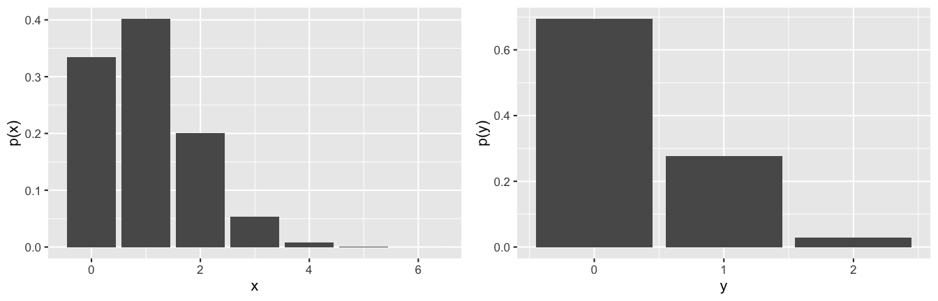
Then the marginal models of $X$ and $Y$ are

\[p_X(x) = P(X = x) \;\; \text{ and } \;\; p_Y(y) = P(Y = y)\]

In tables:

$x$	0	1	2	…	6	Total
$p_X(x)$	$p_X(0)$	$p_X(1)$	$p_X(2)$	…	$p_X(6)$	1
\

$y$	0	1	2	Total
$p_Y(y)$	$p_Y(0)$	$p_Y(1)$	$p_Y(2)$	1

In pictures:

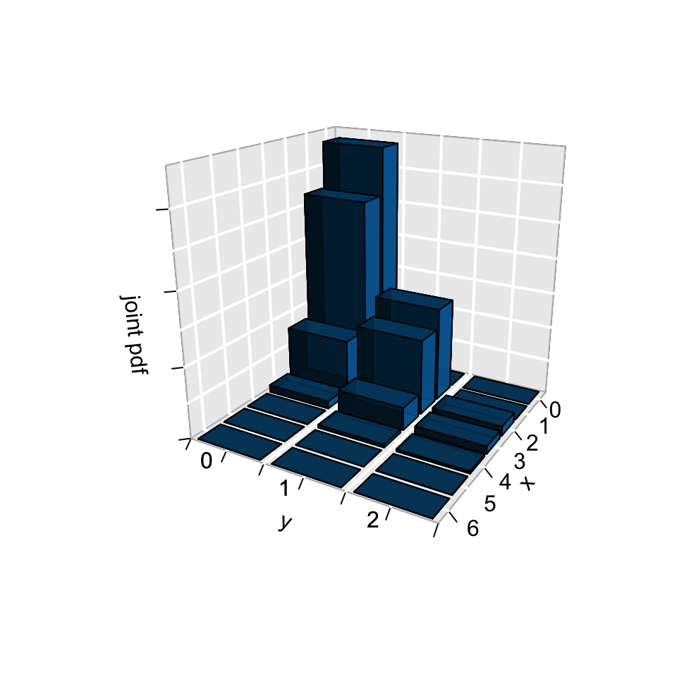
EXAMPLE 2: Joint behavior

\[p_{X,Y}(x,y) = P((X = x) \cap (Y = y))\]

In a table:

$p_{X,Y}(x,y)$	0	$y$ 1	2	Total
0	$p_{X,Y}(0,0)$	$p_{X,Y}(0,1)$	$p_{X,Y}(0,2)$	$p_X(0)$
1	$p_{X,Y}(1,0)$	$p_{X,Y}(1,1)$	$p_{X,Y}(1,2)$	$p_X(1)$
2	$p_{X,Y}(2,0)$	$p_{X,Y}(2,1)$	$p_{X,Y}(2,2)$	$p_X(2)$
3	$p_{X,Y}(3,0)$	$p_{X,Y}(3,1)$	$p_{X,Y}(3,2)$	$p_X(3)$
4	$p_{X,Y}(4,0)$	$p_{X,Y}(4,1)$	$p_{X,Y}(4,2)$	$p_X(4)$
5	$p_{X,Y}(5,0)$	$p_{X,Y}(5,1)$	$p_{X,Y}(5,2)$	$p_X(5)$
6	$p_{X,Y}(6,0)$	$p_{X,Y}(6,1)$	$p_{X,Y}(6,2)$	$p_X(6)$
Total	$p_{Y}(0)$	$p_{Y}(1)$	$p_{Y}(2)$	1

In pictures:

Joint models - Discrete RVs

The simultaneous behavior of $X$ and $Y$ is described by their joint pmf \[p_{X,Y}(x,y) = P(\{X=x\} \cap \{Y=y\}) = P(X=x, Y=y) \;\; \text{(shorthand)}\] where

$p_{X,Y}(x,y) \ge 0$ for all $x,y$

$\sum_x\sum_y p_{X,Y}(x,y) = 1$

Given the joint behavior of $X$ & $Y$, we can find their marginal behaviors using the Law of Total Probability!: \[\begin{split} p_X(x) & = \sum_{all \; y} p_{X,Y}(x,y) \\ p_Y(y) & = \sum_{all \; x} p_{X,Y}(x,y) \\ \end{split}\]

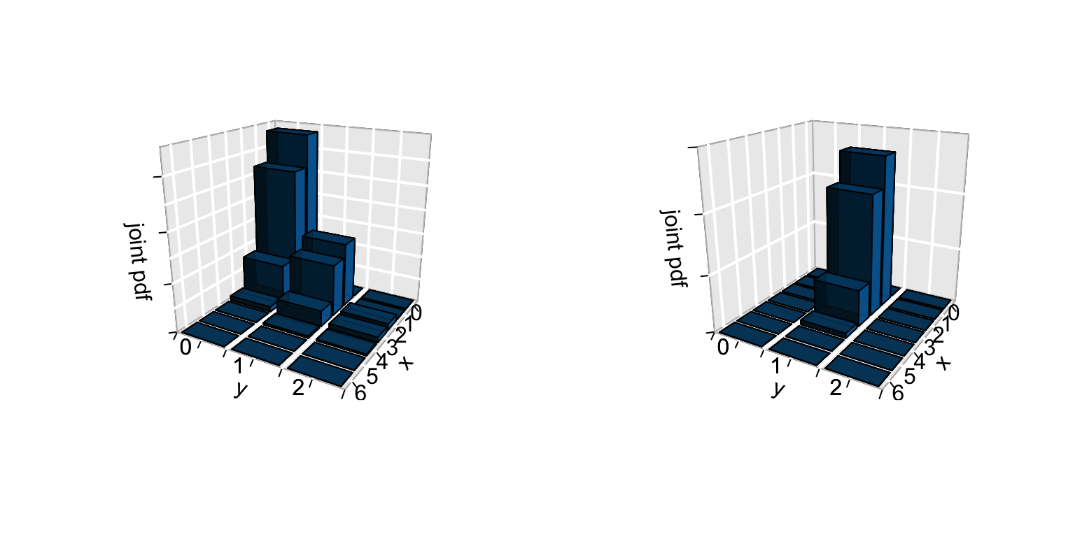
EXAMPLE: Conditional behavior

I tell you that when I rolled the die 6 times, there was one 4 in the first two rolls. The spirit of the conditional pdf of $X$, the number of 4’s in all 6 rolls, given this information is illustrated below:

\[p_{X|(Y=1)}(x|(y=1)) = P(X=x \; | \; Y=1)\]

Conditional models - Discrete RVs

The conditional behavior of $Y$ given that we observe $X=x$ is described by the conditional pmf \[p_{Y|X=x}(y|x) = P(Y=y | X=x)\] where

$p_{Y|X=x}(y|x) \ge 0$ for all $x,y$

$\sum_y p_{Y|X=x}(y|x) = 1$

Given the joint & marginal behaviors of $X$ & $Y$, we can find their conditional behaviors: \[\begin{split} p_{Y|X=x}(y|x) = P(Y=y | X=x) & = \frac{P(Y=y,X=x) }{P(X=x)} = \frac{p_{X,Y}(x,y)}{p_X(x)} \end{split}\]

$X$ and $Y$ are independent if and only if \[\begin{split} p_{Y|X=x}(y|x) & = p_Y(y) \\ p_{X,Y}(x,y) & = p_X(x)p_Y(y) \\ \end{split}\]

NOTE: These statements are equivalent. You only need to check one of them!

18.2 Exercises

In the exercises below, you’ll explore joint and conditional models in the following setting. Roll a die six times. Let \[\begin{split} X & = \text{ # of 4's in the 6 rolls} \\ Y & = \text{ # of 4's in the first 2 rolls} \\ \end{split}\]

To build intuition, you’ll also simulate this experiment 10,000 times and record the observed $X$ and $Y$ for each experiment. There are many more efficient ways to do this, but the following might be more easy to follow:

# Load packages
library(dplyr)
library(janitor)
library(ggplot2)

# Set up the die
die <- c(1:6)

# Set the seed
set.seed(354)

# Simulate the experiment 10000 times
results <- data.frame(
  roll_1 = sample(die, size = 10000, replace = TRUE), 
  roll_2 = sample(die, size = 10000, replace = TRUE), 
  roll_3 = sample(die, size = 10000, replace = TRUE), 
  roll_4 = sample(die, size = 10000, replace = TRUE), 
  roll_5 = sample(die, size = 10000, replace = TRUE), 
  roll_6 = sample(die, size = 10000, replace = TRUE)) %>% 
  mutate(x = (roll_1 == 4) + (roll_2 == 4) + (roll_3 == 4) + (roll_4 == 4) + (roll_5 == 4) + (roll_6 == 4)) %>% 
  mutate(y = (roll_1 == 4) + (roll_2 == 4))

Check out the first 6 experiments. Confirm your understanding of what’s being recorded:

head(results, 6)
##   roll_1 roll_2 roll_3 roll_4 roll_5 roll_6 x y
## 1      6      3      5      5      2      4 1 0
## 2      3      2      1      1      5      1 0 0
## 3      5      5      1      3      1      2 0 0
## 4      3      3      4      1      1      5 1 0
## 5      1      5      1      1      1      4 1 0
## 6      4      3      6      3      1      4 2 1

Marginal models: Simulation
Examine the marginal behavior of $X$ alone and $Y$ alone:

# Table summaries
results %>% 
  tabyl(x)
results %>% 
  tabyl(y)

# Graphical summaries
library(ggplot2)
ggplot(results, aes(x = x)) + 
    stat_count()
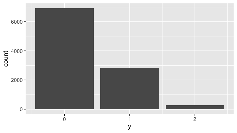
ggplot(results, aes(x = y)) + 
    stat_count()

Solution

# Table summaries
results %>% 
  tabyl(x)
##  x    n percent
##  0 3419  0.3419
##  1 3982  0.3982
##  2 1992  0.1992
##  3  519  0.0519
##  4   86  0.0086
##  5    2  0.0002
results %>% 
  tabyl(y)
##  y    n percent
##  0 6916  0.6916
##  1 2814  0.2814
##  2  270  0.0270

# Graphical summaries
library(ggplot2)
ggplot(results, aes(x = x)) + 
    stat_count()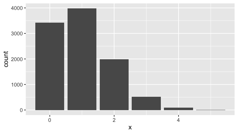

ggplot(results, aes(x = y)) + 
    stat_count()

Joint model: Simulation
Examine the joint behavior of $X$ and $Y$. Be sure to note that the grand table sum is 1 that the row & column sums correspond to the marginal models of $X$ and $Y$!

# Table summaries
results %>% 
  tabyl(x, y) %>% 
  adorn_percentages("all") %>% 
  adorn_totals(c("row", "col"))

# Graphical summary
ggplot(results, aes(x = x, fill = as.factor(y))) +    
    stat_count(position = position_dodge(preserve = "single"))

# 3D plot summary
library(plot3D)
x <- c(0:6)
y <- c(0:2)
p_xy <- function(x,y){choose(2,y)*choose(4,x-y)*(1/6)^x*(5/6)^(6-x)}
z <- outer(x, y, p_xy)
hist3D (x = x, y = y, z = z, 
  bty = "g", phi = 20, theta = 120, 
  xlab = "x", ylab = "y", zlab = "p(x,y)", main = "", 
  col = "#0072B2", border = "black", shade = 0.8,  
  ticktype = "detailed", space = 0.15, d = 2, cex.axis = 1e-9,
  alpha=0.8, zlim=c(0,0.35))
text3D(x = rep(7, 3), y = 0:2, z = rep(0, 3), 
 labels = c("0","1","2"), add = TRUE, adj = 1)
text3D(x = 0:6, y = rep(3,7), z = rep(0, 7), 
 labels = c("0","1","2","3","4","5","6"), add = TRUE, adj = 2.5)

Solution

# Table summaries
results %>% 
  tabyl(x, y) %>% 
  adorn_percentages("all") %>% 
  adorn_totals(c("row", "col"))
##      x      0      1      2  Total
##      0 0.3419 0.0000 0.0000 0.3419
##      1 0.2627 0.1355 0.0000 0.3982
##      2 0.0764 0.1097 0.0131 0.1992
##      3 0.0098 0.0319 0.0102 0.0519
##      4 0.0008 0.0043 0.0035 0.0086
##      5 0.0000 0.0000 0.0002 0.0002
##  Total 0.6916 0.2814 0.0270 1.0000

# Graphical summary
ggplot(results, aes(x = x, fill = as.factor(y))) +    
    stat_count(position = position_dodge(preserve = "single"))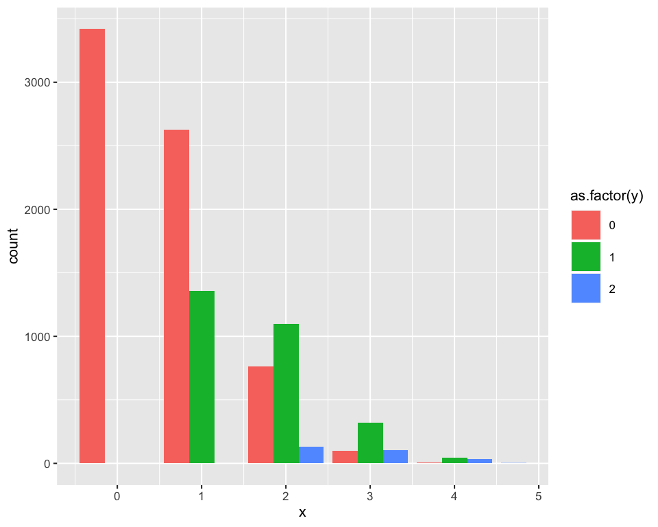


# 3D plot summary
library(plot3D)
x <- c(0:6)
y <- c(0:2)
p_xy <- function(x,y){choose(2,y)*choose(4,x-y)*(1/6)^x*(5/6)^(6-x)}
z <- outer(x, y, p_xy)
hist3D (x = x, y = y, z = z, 
  bty = "g", phi = 20, theta = 120, 
  xlab = "x", ylab = "y", zlab = "p(x,y)", main = "", 
  col = "#0072B2", border = "black", shade = 0.8,  
  ticktype = "detailed", space = 0.15, d = 2, cex.axis = 1e-9,
  alpha=0.8, zlim=c(0,0.35))
text3D(x = rep(7, 3), y = 0:2, z = rep(0, 3), 
 labels = c("0","1","2"), add = TRUE, adj = 1)
text3D(x = 0:6, y = rep(3,7), z = rep(0, 7), 
 labels = c("0","1","2","3","4","5","6"), add = TRUE, adj = 2.5)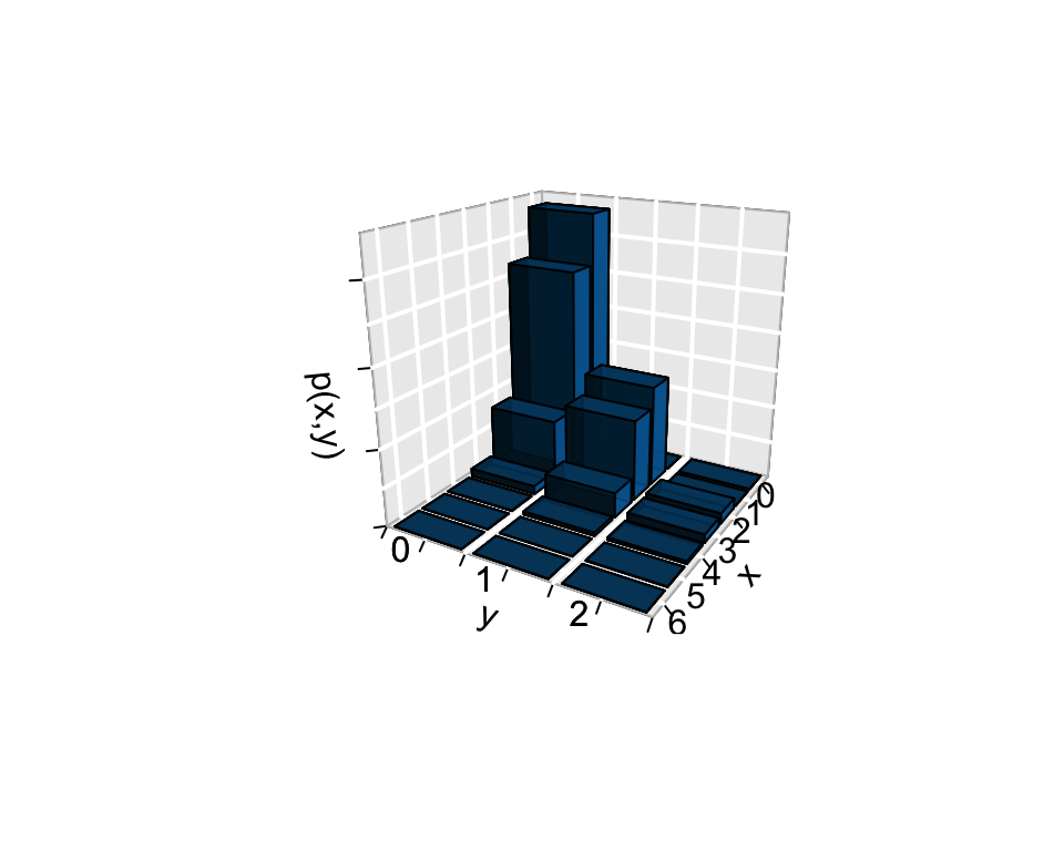

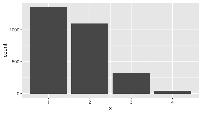
Conditional model: simulation
Suppose I tell you $Y = 1$. Examine the conditional behavior of $X$ given this information. Note that within the world where $Y = 1$, the model of $X$ is valid – the conditional pmf sums to 1.

# Restrict the sample space
y_1 <- results %>% 
  filter(y == 1)

# Table summary
y_1 %>% 
  tabyl(x)

# Graphical summary
ggplot(y_1, aes(x = x)) +    
    stat_count()

Solution

# Restrict the sample space
y_1 <- results %>% 
  filter(y == 1)

# Table summary
y_1 %>% 
  tabyl(x)
##  x    n    percent
##  1 1355 0.48152097
##  2 1097 0.38983653
##  3  319 0.11336176
##  4   43 0.01528074

# Graphical summary
ggplot(y_1, aes(x = x)) +    
    stat_count()

Marginal models: Math
a. Convince yourself that $X \sim Bin(6,1/6)$ and $Y \sim Bin(2,1/6)$. Thus \[\begin{split} p_{X}(x) & = \left( \begin{array}{c} 6 \\x \end{array} \right)\frac{1}{6}^x \frac{5}{6}^{6-x} \;\; \text{ for } x \in \{0,1,2,3,4,5,6\} \\ p_{Y}(y) & = \left( \begin{array}{c} 2 \\y \end{array} \right)\frac{1}{6}^y \frac{5}{6}^{2-y} \;\; \text{ for } y \in \{0,1,2\} \\ \end{split}\]

b. For peace of mind, confirm at least one calculation in each of the following tables.  The Monte Carlo simulation results from exercise 1 should be very similar!

c. Confirm that $E(X) = 1$.

$x$	0	1	2	3	4	5	6	Total
$p_X(x)$	0.33490	0.40188	0.20094	0.05358	0.00804	0.00064	0.00002	1

$y$	0	1	2	Total
$p_Y(y)$	0.69444	0.27778	0.02778	1

Solution

Yes. Both $X$ and $Y$ are the number of successes in a fixed number of independent trials, each trial having the same probability of success.
$p_X(0) = \left( \begin{array}{c} 6 \\ 0\end{array} \right)\frac{1}{6}^0 \frac{5}{6}^{6-0} = 0.3349$
$X \sim Bin(6,1/6)$, thus $E(X) = 6*1/6 = 1$

Joint model: Math

Build a formula for the joint pmf of $X$ and $Y$. Be careful with the support! HINT: The answer is revealed in exercise 6 if you get stuck. \[\begin{split} p_{X,Y}(x,y) & = P(X=x,Y=y) = ??? \end{split}\]

For peace of mind, confirm at least one calculation in the following table. The Monte Carlo simulation results from exercise 2 should be very similar!

$p_{X,Y}(x,y)$	0	$y$ 1	2	Total
0	0.334898	0	0	0.33490
1	0.267917	0.133960	0	0.40188
2	0.080376	0.107167	0.013396	0.20094
3	0.010717	0.032150	0.010717	0.05358
4	0.000536	0.004287	0.003215	0.00804
5	0	0.000214	0.000429	0.00064
6	0	0	0.000021	0.00002
Total	0.69444	0.2778	0.02778	1

Solution

For $y \in \{0,1,2\}, x \in \{y,...,y+4\}$, \[\begin{split} p_{X,Y}(x,y) & = P(y \text{ 4's in first 2 }, x-y \text{ in last 4}) \\ & = \left( \begin{array}{c} 2 \\y \end{array} \right) \frac{1}{6}^y \frac{5}{6}^{2-y} \cdot \left( \begin{array}{c} 4 \\x-y \end{array} \right) \frac{1}{6}^{x-y} \frac{5}{6}^{4-x+y} \\ & = \left( \begin{array}{c} 2 \\y \end{array} \right) \left( \begin{array}{c} 4 \\x-y \end{array} \right) \frac{1}{6}^x \frac{5}{6}^{6-x}\\ \end{split}\]

Conditional model: math
Above you built the marginal and joint models of $X$ and $Y$:

\[\begin{split} p_{X}(x) & = \left( \begin{array}{c} 6 \\x \end{array} \right)\frac{1}{6}^x \frac{5}{6}^{6-x} \;\; \text{ for } x \in \{0,1,2,3,4,5,6\} \\ p_{Y}(y) & = \left( \begin{array}{c} 2 \\y \end{array} \right)\frac{1}{6}^y \frac{5}{6}^{2-y} \;\; \text{ for } y \in \{0,1,2\} \\ p_{X,Y}(x,y) & = \left( \begin{array}{c} 2 \\y \end{array} \right) \left( \begin{array}{c} 4 \\x-y \end{array} \right) \left(\frac{1}{6}\right)^x \left(\frac{5}{6}\right)^{6-x} \;\; \text{ for } y \in \{0,1,2\}, x \in \{y,...,y+4\} \\ \end{split}\]
1. Suppose I tell you that I rolled a die 6 times and there was one 4 in the first two rolls ($Y = 1$). Build the conditional pmf of $X$, the number of 4’s in all 6 rolls, given this information: \[p_{X|(Y=1)}(x|(y=1)) = P(X=x | Y=1) = ???\]
2. For peace of mind, using your formula from part a, confirm at least one of the calculations in the following table:
  
  $x$ 1 2 3 4 5 Total
  
  $p_{X|(Y=1)}(x|(y=1))$ 0.482 0.386 0.116 0.015 0.001 1
3. Further, re-examine the table of the joint pmf $p_{X,Y}(x,y)$. Confirm that $p_{X|(Y=1)}((x=1)|(y=1)) = 0.482$ using the joint table as opposed to the formula from part a.
4. Calculate $E(X|(Y=1))$ and compare this to $E(X) = 1$.
Solution
1. .
  
  \[\begin{split} p_{X|(Y=1)}(x|(y=1)) & = \frac{p_{X,Y}(x,1)}{p_Y(1)} \\ & = \frac{\left( \begin{array}{c} 2 \\ 1 \end{array} \right) \left( \begin{array}{c} 4 \\x - 1 \end{array} \right) \left(\frac{1}{6}\right)^x \left(\frac{5}{6}\right)^{6-x}}{\left( \begin{array}{c} 2 \\1 \end{array} \right)\frac{1}{6}^1 \frac{5}{6}^{2-1} } \\ & = \frac{\left( \begin{array}{c} 4 \\x - 1 \end{array} \right) \left(\frac{1}{6}\right)^x \left(\frac{5}{6}\right)^{6-x}}{\frac{1}{6} \frac{5}{6} } \\ & = \left( \begin{array}{c} 4 \\x - 1 \end{array} \right) \left(\frac{1}{6}\right)^{x-1} \left(\frac{5}{6}\right)^{5-x} \\ \end{split}\]
2. .
  \[\begin{split} p_{X|(Y=1)}((x=1)|(y=1)) & = \left( \begin{array}{c} 4 \\ 1 - 1 \end{array} \right) \left(\frac{1}{6}\right)^{1-1} \left(\frac{5}{6}\right)^{5-1} \\ & = \left(\frac{5}{6}\right)^{4} \\ & \approx 0.482 \\ \end{split}\]
3. $0.133960/0.2778 \approx 0.482$
4. $E(X|(Y=1)) = 1*.482 + 2*.386 + 3*0.116 + 4*0.015 + 5*0.001 = 1.667$
  Knowing that we already got 1 4 in the first 2 rolls, we expect more 4’s overall (relative to when we don’t know what happened in the first 2 rolls).

\(x\)	1	2	3	4	5	Total
\(p_{X\|(Y=1)}(x\|(y=1))\)	0.482	0.386	0.116	0.015	0.001	1

General conditional model
1. In general, suppose I tell you that I rolled a die 6 times and there were $y$ 4’s in the first two rolls. Calculate the conditional pmf of $X$ given this information. (Does this make intuitive sense now that you see the formula?!?) \[p_{X|(Y=y)}(x|y) = P(X=x | Y=y) = ???\]
2. CHALLENGE (give it a try): Prove that this is a valid conditional pmf.
3. CHALLENGE (give it a try): Provide a general formula for $E(X|(Y=y))$.
Solution
1. For $x \in \{y,...,y+4\}$,
  \[\begin{split} p_{X|(Y=y)}(x|y) & = \frac{p_{X,Y}(x,y)}{p_Y(y)} \\ & = \frac{\left( \begin{array}{c} 2 \\ y \end{array} \right) \left( \begin{array}{c} 4 \\ x - y \end{array} \right) \left(\frac{1}{6}\right)^x \left(\frac{5}{6}\right)^{6-x}}{\left( \begin{array}{c} 2 \\ y \end{array} \right)\frac{1}{6}^y \frac{5}{6}^{2-y} } \\ & = \frac{\left( \begin{array}{c} 4 \\x - y \end{array} \right) \left(\frac{1}{6}\right)^x \left(\frac{5}{6}\right)^{6-x}}{\frac{1}{6}^y \frac{5}{6}^{2-y} } \\ & = \left( \begin{array}{c} 4 \\ x - y \end{array} \right) \left(\frac{1}{6}\right)^{x-y} \left(\frac{5}{6}\right)^{4-(x-y)} \\ \end{split}\]
2. .
  \[\begin{split} \sum_{x = y}^{y+4}p_{X|(Y=y)}(x|y) & = \sum_{x = y}^{y+4}\left( \begin{array}{c} 4 \\ x - y \end{array} \right) \left(\frac{1}{6}\right)^{x-y} \left(\frac{5}{6}\right)^{4-(x-y)} \\ & = \sum_{z = 0}^{4}\left( \begin{array}{c} 4 \\ z \end{array} \right) \left(\frac{1}{6}\right)^{z} \left(\frac{5}{6}\right)^{4-z} \;\;\; \text{(letting $z = x-y$)} \\ & = \sum_{z = 0}^{4} \text{pmf of a Bin(4, 1/6)} \\ & = 1 \\ \end{split}\]
3. FUN!
  \[\begin{split} E(X|(Y=y)) & = \sum_{x = y}^{y+4}x*p_{X|(Y=y)}(x|y) & = \sum_{x = y}^{y+4}x*\left( \begin{array}{c} 4 \\ x - y \end{array} \right) \left(\frac{1}{6}\right)^{x-y} \left(\frac{5}{6}\right)^{4-(x-y)} \\ & = \sum_{z = 0}^{4}(z+y)*\left( \begin{array}{c} 4 \\ z \end{array} \right) \left(\frac{1}{6}\right)^{z} \left(\frac{5}{6}\right)^{4-z} \;\;\; \text{(letting $z = x-y$)} \\ & = \sum_{z = 0}^{4} (z + y) * (\text{pmf of a Bin(4, 1/6)}) \\ & = \sum_{z = 0}^{4} z * (\text{pmf of a Bin(4, 1/6)}) + y \sum_{z = 0}^{4} (\text{pmf of a Bin(4, 1/6)}) \\ & = E(\text{a Bin(4, 1/6) RV}) + y*1 \\ & = 4*1/6 + y \\ & = 2/3 + y \\ \end{split}\]

Independence
1. In the dice experiment, are $X$ and $Y$ independent? Provide proof.
2. Consider an apartment with 2 student roommates. Let $X$ be the number of these students that are taking at least 1 MSCS class and $Y$ be the number that like pizza. Based on the following table, are $X$ and $Y$ independent?

$p_{X,Y}(x,y)$	0	$y$ 1	2	Total
0	0.0075	0.0675	0.6750	0.75
1	0.0020	0.0180	0.1800	0.20
2	0.0005	0.0045	0.0450	0.05
Total	0.0100	0.09	0.90	1

Solution

No. $p_{X|Y}(x|y) \ne p_X(x)$. Knowing what happens in the first 2 rolls ($Y$) tells us something about what happens overall ($X$).
Yes. Every joint entry is a product of the marginals, $p(x,y) = p(x)p(y)$.

\(x\)	0	1	2	…	6	Total
\(p_X(x)\)	\(p_X(0)\)	\(p_X(1)\)	\(p_X(2)\)	…	\(p_X(6)\)	1
\

\(p_{X,Y}(x,y)\)	0	\(y\) 1	2	Total
0	\(p_{X,Y}(0,0)\)	\(p_{X,Y}(0,1)\)	\(p_{X,Y}(0,2)\)	\(p_X(0)\)
1	\(p_{X,Y}(1,0)\)	\(p_{X,Y}(1,1)\)	\(p_{X,Y}(1,2)\)	\(p_X(1)\)
2	\(p_{X,Y}(2,0)\)	\(p_{X,Y}(2,1)\)	\(p_{X,Y}(2,2)\)	\(p_X(2)\)
3	\(p_{X,Y}(3,0)\)	\(p_{X,Y}(3,1)\)	\(p_{X,Y}(3,2)\)	\(p_X(3)\)
4	\(p_{X,Y}(4,0)\)	\(p_{X,Y}(4,1)\)	\(p_{X,Y}(4,2)\)	\(p_X(4)\)
5	\(p_{X,Y}(5,0)\)	\(p_{X,Y}(5,1)\)	\(p_{X,Y}(5,2)\)	\(p_X(5)\)
6	\(p_{X,Y}(6,0)\)	\(p_{X,Y}(6,1)\)	\(p_{X,Y}(6,2)\)	\(p_X(6)\)
Total	\(p_{Y}(0)\)	\(p_{Y}(1)\)	\(p_{Y}(2)\)	1