23 Sampling distributions: min, max, sum

23.1 Discussion

Recall

In the previous activity, we studied iid samples of size \(n\) from the Exp(1) model:

\[(X_1,X_2,...,X_n) \stackrel{ind}{\sim} Exp(1)\]

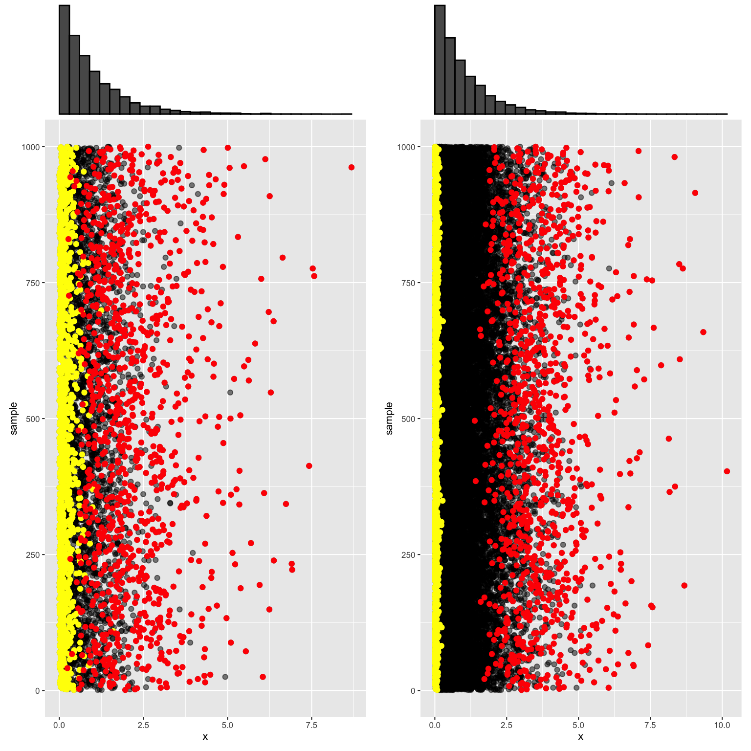
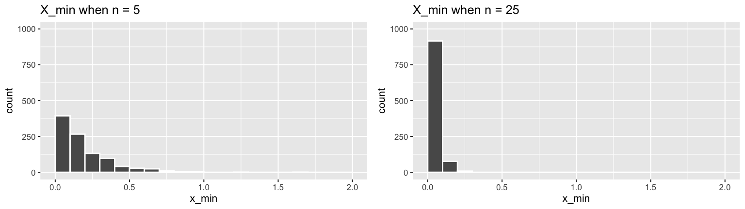
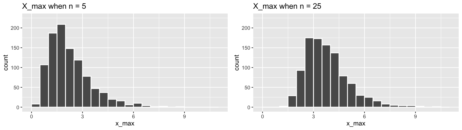
Below are 1000 samples of size \(n = 5\) (left) and 1000 samples of size \(n = 25\) (right). Through this simulation, we can study the variability in \(X_{min}\) (yellow) and \(X_{max}\) (red) from sample to sample as well as how this variability is impacted by sample size \(n\).

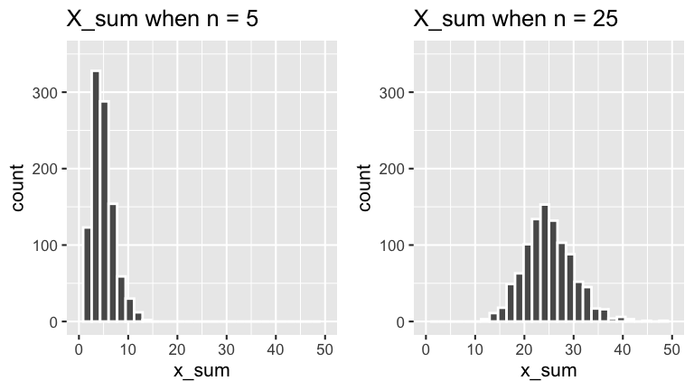
We also simulated the variability in \(X_{sum}\):

Goal

The simulations above help us approximate the sampling distributions (probability models) of \(X_{min}\), \(X_{max}\), and \(X_{sum}\). In this activity we’re going to build the theory behind these models!

EXAMPLE 1: getting ready

In order to do study sample sum \(X_{sum}\), we need an understanding of how expected values and variances work for sums of random variables. To this end, let \(X,Y\) be independent RVs, thus

\[f_{X,Y}(x,y) = f_X(x)f_Y(y)\]
Further, show that

\[\begin{split} E(aX + bY) & = aE(X) + bE(Y) \\ Var(aX + bY)& = a^2Var(X) + b^2Var(Y) \\ E(g(X)h(Y)) & = E(g(X))E(h(Y)) \;\; \text{ for functions } g(), h() \\ \end{split}\]

In doing so, assume \(X,Y\) are continuous. The discrete proof is similar.

Solution

\[\begin{split} E(aX + bY) & = \int\int (ax + by)f_{X,Y}(x,y)dxdy \\ & = \int\int (ax + by)f_{X}(x)f_Y(y)dxdy \\ & = a\int\int xf_{X}(x)f_Y(y)dxdy + b\int\int yf_{X}(x)f_Y(y)dxdy \\ & = a\int\left[\int xf_{X}(x)dx\right]f_Y(y)dy + b\int\left[yf_Y(y) \int f_{X}(x)dx\right]dy \\ & = a E(X)\int f_Y(y)dy + b\int yf_Y(y)dy \\ & = a E(X) + bE(Y) \\ Var(aX + bY) & = E\left[\left((aX+bY) - E(aX+bY)\right)^2\right] \\ & = E\left[\left(aX+bY - aE(X) - bE(Y)\right)^2\right] \\ & = E\left[\left(a(X-E(X)) + b(Y - E(Y))\right)^2\right] \\ & = E\left[a^2(X-E(X))^2 + b^2(Y - E(Y))^2 + 2ab(X-E(X))(Y-E(Y))\right] \\ & = a^2E[(X-E(X))^2] + b^2E[(Y - E(Y))^2] + 2abE[(X-E(X))(Y-E(Y))] \\ & = a^2Var(X) + b^2Var(Y) + 2abE[X-E(X)]E[Y-E(Y)] \\ & = a^2Var(X) + b^2Var(Y) \\ E(g(X)h(Y)) & = \int_y\int_xg(x)h(y)f_{X,Y}(x,y)dxdy\\ & = \int_y\int_xg(x)h(y)f_X(x)f_Y(y)dxdy\\ & = \left[\int_yh(y)f_Y(y)dy\right]\left[\int_xg(x)f_X(x)dx\right]\\ & = E(g(X))E(h(Y)) \\ \end{split}\]

23.2 Exercises

23.2.1 Minimum & maximum

Uniform setting
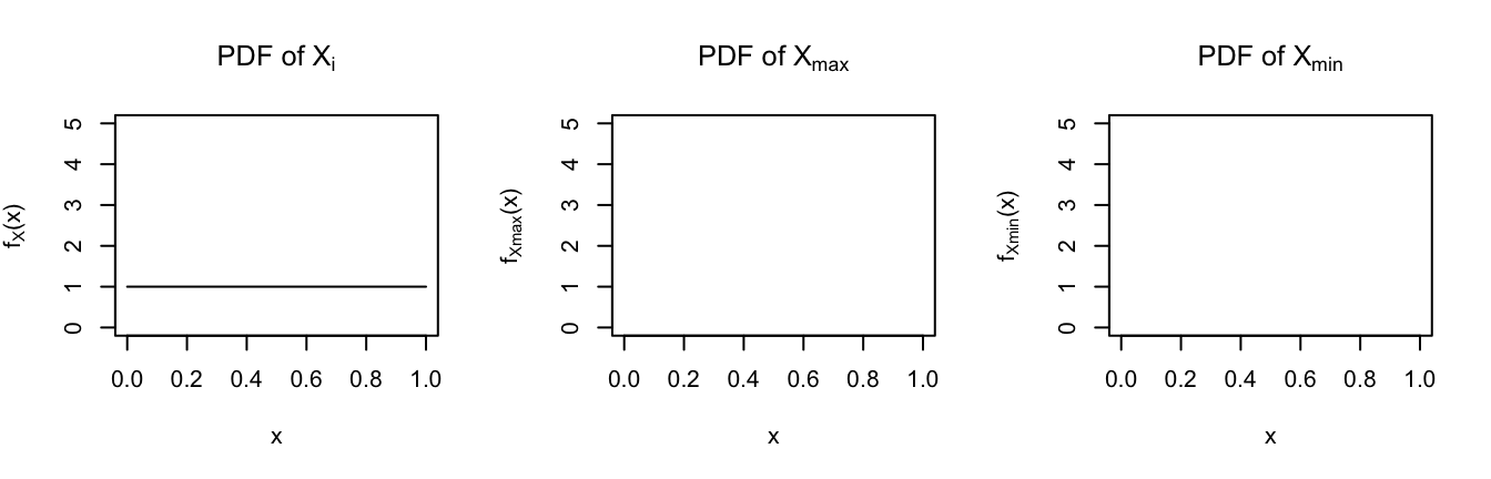
Forget the exponential lightbulbs for now. Let’s play a game in which we draw an iid sample of \(n\) numbers (\(X_1,X_2,...,X_n\)) from the \(Unif(0,1)\) population with

\[\begin{split} f_X(x) & = 1 \;\; \text{ for } x \in [0,1] \\ F_X(x) & = \begin{cases} 0 & x < 0 \\ x & 0 \le x < 1 \\ 1 & x \ge 1 \\ \end{cases} \\ \end{split}\]

Let \(X_{min}\) and \(X_{max}\) denote the minimum and maximum values of this sample.
1. Which of the following statement(s) are true:
  - \(X_{min} \le x\) if and only if all \(X_i \le x\)
  - \(X_{max} \le x\) if and only if all \(X_i \le x\)
  - \(X_{min} > x\) if and only if all \(X_i > x\)
  - \(X_{max} > x\) if and only if all \(X_i > x\)
2. Which of the following statement(s) are true:
  - \(P(X_{min} \le x) = P(X_1 \le x)P(X_2 \le x) \cdots P(X_n \le x)\)
  - \(P(X_{max} \le x) = P(X_1 \le x)P(X_2 \le x) \cdots P(X_n \le x)\)
  - \(P(X_{min} > x) = P(X_1 > x)P(X_2 > x) \cdots P(X_n > x)\)
  - \(P(X_{max} > x) = P(X_1 > x)P(X_2 > x) \cdots P(X_n > x)\)
Solution
1. \(X_{min} \le x\) if and only if all \(X_i \le x\)
  \(X_{min} > x\) if and only if all \(X_i > x\)
2. \(P(X_{max} \le x) = P(X_1 \le x)P(X_2 \le x) \cdots P(X_n \le x)\)
  \(P(X_{min} > x) = P(X_1 > x)P(X_2 > x) \cdots P(X_n > x)\)

Uniform with \(n=2\)
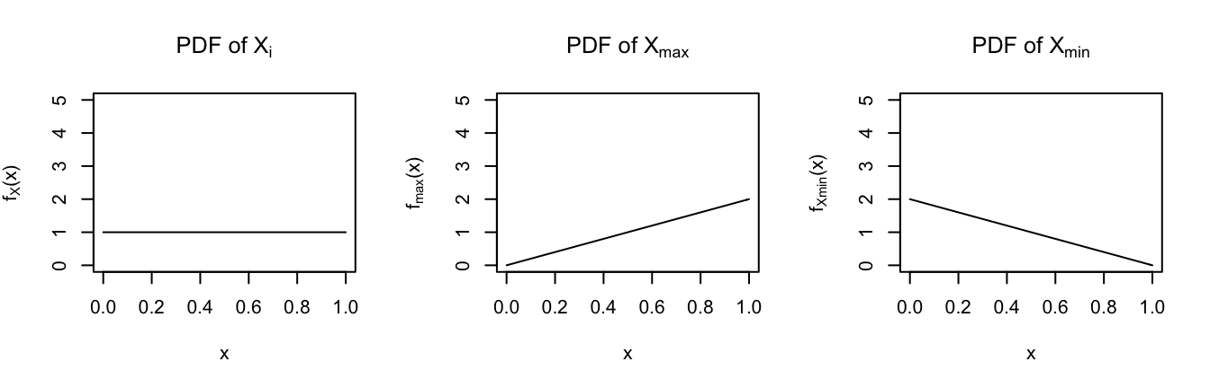
Start by assuming that we have a small sample size with \(n=2\), (\(X_1,X_2\)), from the Unif(0,1) model. In completing this exercise, utilize your answer to exercise 1 and remember that the \(X_i\) are continuous.
1. For this simplified setting with \(n=2\), derive the PDF for \(X_{max}\), \(f_{X_{max}}(x)\).
  Hint
  
  Start with
  
  \[F_{X_{max}}(x) = P(X_{max} \le x) = P(X_1 \le t)P(X_2 \le t)\]
  
  Then get
  \[f_{X_{max}}(x) = \frac{d}{dx}F_{X_{max}}(x)\]
2. For this simplified setting with \(n=2\), derive the PDF for \(X_{min}\), \(f_{X_{min}}(x)\).
  Hint
  
  Start with
  
  \[\begin{split} F_{X_{min}}(x) & = P(X_{min} \le x) \\ & = 1 - P(X_{min} > x) \\ & = 1 - P(X_1 > x)P(X_2 > x) \\ \end{split}\]
  
  Then get
  \[f_{X_{min}}(x) = \frac{d}{dx}F_{X_{min}}(x)\]
3. Sketch the PDFs of \(X_{max}\) and \(X_{min}\).
Solution
1. For \(x \in (0,1)\), \[\begin{split} F_{X_{max}}(x) & = P(X_{max} \le x) \\ & = P(X_1 \le x)P(X_2 \le x) \\ & = F_{X}(t)F_{X}(t)\\ & = t^2 \\ f_{X_{max}}(x) & = \frac{d}{dx}F_{X_{max}}(x) = 2x \\ \end{split}\]
2. For \(x \in (0,1)\), \[\begin{split} F_{X_{min}}(x) & = P(X_{min} \le x) \\ & = 1 - P(X_{min} > x) \\ & = 1 - P(X_1 > x)P(X_2 > x) \\ & = 1 - (1 - F_X(x))(1 - F_X(x)) \\ & = 1 - (1 - x)(1 - x) \\ & = 1 - (1-x)^2 \\ f_{X_{min}}(x) & = \frac{d}{dx}F_{X_{min}}(x) = 2(1-x) \\ \end{split}\]
3. .

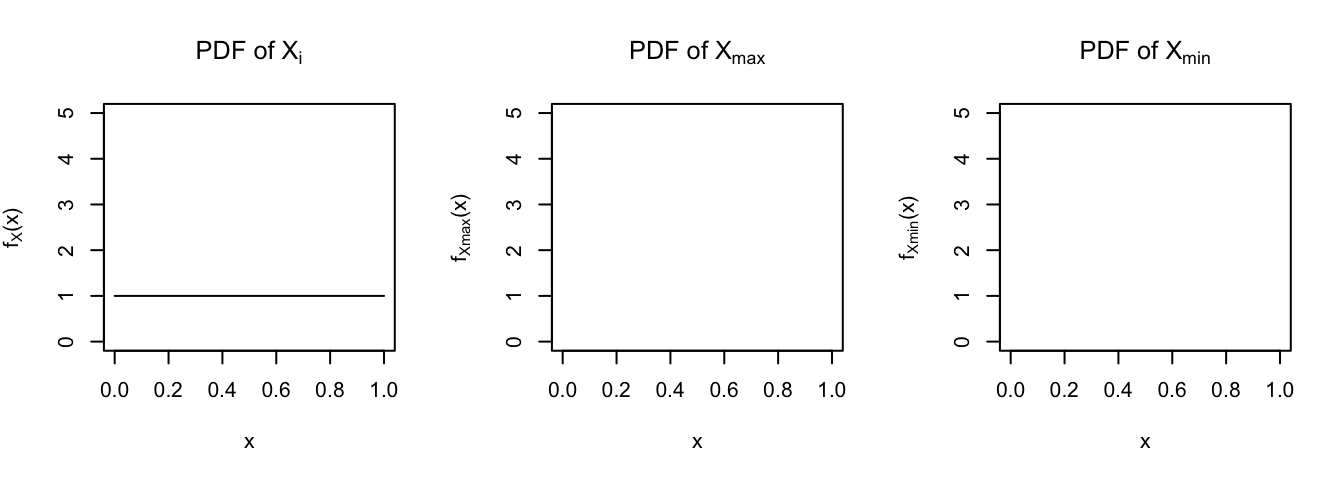
Uniform with \(n=5\)
Next, suppose we have a increase our sample size from the Unif(0,1) to \(n=5\): (\(X_1,X_2,...,X_5\)).
1. Derive the PDF for \(X_{max}\), \(f_{X_{max}}(x)\).
2. Derive the PDF for \(X_{min}\), \(f_{X_{min}}(x)\).
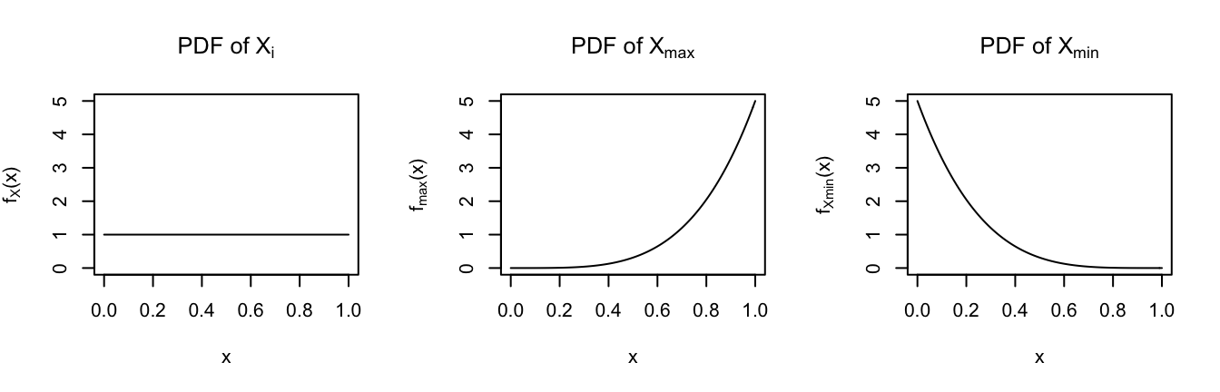
3. Sketch the PDFs of \(X_{max}\) and \(X_{min}\) in the frames below.
Solution
1. For \(x \in (0,1)\), \[\begin{split} F_{X_{max}}(x) & = P(X_{max} \le x) \\ & = P(X_1 \le x)P(X_2 \le x) \cdots P(X_5 \le x) \\ & = x^5 \\ f_{X_{max}}(x) & = \frac{d}{dx}F_{X_{max}}(x) = 5x^4 \\ \end{split}\]
2. For \(x \in (0,1)\), \[\begin{split} F_{X_{min}}(x) & = P(X_{min} \le x) \\ & = 1 - P(X_{min} > x) \\ & = 1 - P(X_1 > x)P(X_2 > x)\cdots P(X_5 > x) \\ & = 1 - (1 - F_X(x))(1 - F_X(x)) \cdots (1-F_X(x)) \\ & = 1 - (1 - x)^5 \\ f_{X_{min}}(x) & = \frac{d}{dx}F_{X_{min}}(x) = 5(1-x)^4 \\ \end{split}\]
3. .

Reflection
Summarize your observations from the above 2 exercises. Specifically, comment on how the models of \(X_{min}\) & \(X_{max}\) compare to that of \(X_i\) AND how sample size \(n\) impacts these models.

Solution
\(X_{min}\) is more likely to be close to 0 and \(X_{max}\) is more likely to be close to 1 in comparison to just the single value of one of the sample draws \(X\). As sample size \(n\) increases, \(X_{min}\) is drawn closer and closer to 0 and \(X_{max}\) is drawn closer and closer to 1 – the bigger our sample, the more chances we have to get a really small minimum (near 0) and a really large maximum (near 1).

Generalize it
Let’s extend these ideas to the general setting. Suppose \(X_1,...,X_n\) are iid from some model/population (not necessarily Uniform) with PDF \(f_X(x)\) and cdf \(F_X(x)\).
1. Prove that the PDF of \(X_{max}\) is \[f_{X_{max}}(x) = n [F_X(x)]^{n-1} \cdot f_X(x)\]
2. Similarly, show that the PDF of \(X_{min}\) is \[f_{X_{min}}(x) = n [1-F_X(x)]^{n-1} \cdot f_X(x)\]
Solution

\[\begin{split} F_{X_{min}}(x) & = P(X_{min} \le x) \;\; \text{ (definition)} \\ & = 1 - P(X_{min} > x) \;\; \text{ (complement rule)} \\ & = 1 - P(X_1>x, X_2>x, \ldots, X_n>x) \;\; \text{ (meaning of "minimum")} \\ & = 1 - P(X_1>x)P(X_2>x) \cdots P(X_n>x) \;\; \text{ (independence)} \\ & = 1 - (1-P(X_1\le x))(1-P(X_2\le x)) \cdots (1-P(X_n\le x)) \\ & = 1 - (1-F_X(x))(1-F_X(x)) \cdots (1-F_X(x)) \\ & = 1 - (1 - F_X(x))^n \\ f_{X_{min}}(x) & = \frac{d}{dx}F_{X_{min}}(x) \\ & = \frac{d}{dx} \left[ 1 - (1 - F_X(x))^n \right] \\ & = n [1-F_X(x)]^{n-1} \cdot f_X(x) \;\; \text{ (chain rule)} \\ F_{X_{max}}(x) & = P(X_{max} \le x) \;\; \text{ (definition)} \\ & = P(X_1\le x, X_2 \le x, \ldots, X_n \le x) \;\; \text{ (meaning of "maximum")} \\ & = P(X_1 \le x)P(X_2 \le x) \cdots P(X_n \le x) \;\; \text{ (independence)} \\ & = F_X(x)^n \\ f_{X_{max}}(x) & = \frac{d}{dx}F_{X_{max}}(x) \\ & = \frac{d}{dx} \left[ F_X(x)^n \right] \\ & = n [F_X(x)]^{n-1} \cdot f_X(x) \;\; \text{ (chain rule)} \\ \end{split}\]

Building the sampling distribution of \(X_{min}\) for \(Exp(\lambda)\)
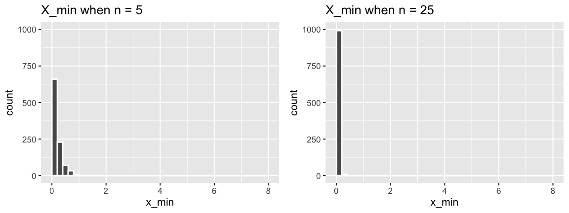
Let’s return to the Exponential model. Recall that \(X_{min}\) exhibited the following behavior across samples of size \(n = 5\) and \(n = 25\):

Let’s support these simulation results with some math! In doing so, consider the general setting in which \((X_1,...,X_n)\), a sample of size \(n\), are iid \(Exp(\lambda)\) with common features:
\[\begin{split} f_X(x) & = \lambda e^{-\lambda x} \hspace{.2in} \text{ for } x > 0 \\ F_X(x) & = 1- e^{-\lambda x} \hspace{.2in} \text{ for } x > 0 \\ M_X(t) & = \frac{\lambda}{\lambda - t} \\ E(X) & = \frac{1}{\lambda}\\ Var(X) & = \frac{1}{\lambda^2}\\ \end{split}\]
1. Provide a formula for the PDF of \(X_{min}\), the shortest waiting time in a random sample. RECALL: \[f_{X_{min}}(x) = n [1-F_X(x)]^{n-1} \cdot f_X(x)\]
2. Identify the model of \(X_{min}\). NOTE: The plots of \(X_{min}\) above should also provide a clue!
Solution
1. .
  \[\begin{split} f_{X_{min}}(x) & = n [1-F_X(x)]^{n-1} \cdot f_X(x) \\ & = n [1-(1- e^{-\lambda x})]^{n-1} \cdot \lambda e^{-\lambda x} \\ & = n [e^{-\lambda x}]^{n-1} \cdot \lambda e^{-\lambda x} \\ & = n e^{-\lambda x (n-1)} \cdot \lambda e^{-\lambda x} \\ & = (n\lambda) e^{-(n\lambda) x} \\ \end{split}\]
2. \(X_{min} \sim Exp(n\lambda)\)

Interpreting the sampling distribution of \(X_{min}\) for \(Exp(\lambda)\)
1. Calculate and compare \(E(X)\) and \(E(X_{min})\).
  - Which is smaller? Why does this make sense?
  - How does \(E(X_{min})\) change as \(n\) increases?
2. Calculate and compare \(Var(X)\) and \(Var(X_{min})\).
  - Which is smaller? Why does this make sense?
  - How does \(Var(X_{min})\) change as \(n\) increases?
3. Recall our sample of 25 lightbulbs where the lifetime of a given bulb is modeled by Exp(1). Thus the expected lifetime of any given bulb is \(E(X) = 1\) year. Specify the model of \(X_{min}\) among the 25 bulbs and calculate \(E(X_{min})\).
Solution
1. \(E(X) = 1/\lambda\), \(E(X_{min}) = 1/(n\lambda)\)
  - \(E(X_{min}) \le E(X)\) which makes sense since the expected minimum among multiple observations should be smaller than the expected value of a single observation.
  - \(E(X_{min})\) decreases as \(n\) increases. This makes sense since as we increase sample size, the more and more likely we are to get a minimum value that’s closer and closer to 0.
2. \(Var(X) = 1/\lambda^2\), \(E(X_{min}) = 1/(n\lambda)^2\)
  - \(Var(X_{min}) \le Var(X)\). This makes sense since there’s more variability among individual observations of \(X\) than among a property that’s calculated across multiple sample observations. That is, there’s more certainty in saying something about group behavior than about individual behavior.
  - \(Var(X_{min})\) decreases as \(n\) increases. This makes sense since as we increase sample size, the more and more the minimum value will stabilize near 0.
3. \(X_{min} \sim Exp(25)\) with \(E(X_{min}) = 1/25\) years.

Sampling distribution of \(X_{max}\) for \(Exp(\lambda)\)
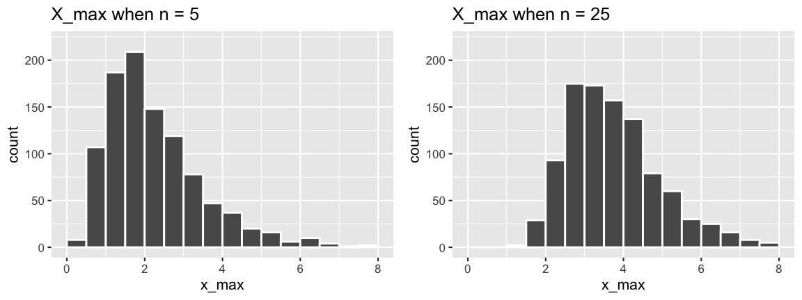
Again, let \((X_1,...,X_n)\) be an iid sample from \(Exp(\lambda)\) with a maximum value of \(X_{max}\). Recall that \(X_{min}\) exhibited the following behavior across samples of size \(n = 5\) and \(n = 25\):
1. Provide a formula for the PDF of \(X_{max}\). RECALL:
  \[f_{X_max}(x) = n [F_X(x)]^{n-1} \cdot f_X(x)\]
2. Does \(X_{max}\) have an exponential model? NOTE: The answer to this question is also evident from the plots of \(X_{max}\) in the discussion section.
Solution
1. .
  \[\begin{split} f_{X_{max}}(x) & = n [F_X(x)]^{n-1} \cdot f_X(x) \\ & = n [1- e^{-\lambda x}]^{n-1} \cdot \lambda e^{-\lambda x} \\ \end{split}\]
2. No. This isn’t an Exponential pdf.

23.2.2 Sums

Properties of a sample sum
NOTE: For this exercise, Example 1 from the discussion section will come in handy!

Let \((X_1,...,X_n)\) be an iid random sample from some model/population. Since the \(X_i\) are drawn from the same model, they have the same pdf \(f_X(x)\), cdf \(F_X(x)\), mgf \(M_X(t)\), mean \(\mu_X = E(X_i)\), and variance \(\sigma^2_X = Var(X_i)\) Let’s examine the basic properties of the sum of this sample

\[X_{sum} = \sum_{i=1}^n X_i\]
1. Provide a formula for \(E(X_{sum})\). This will depend upon \(\mu_X\) and sample size \(n\).
2. Provide a formula for \(Var(X_{sum})\). This will depend upon \(\sigma_X^2\) and sample size \(n\).
3. Prove that the MGF of \(X_{sum}\) is a function of the MGF of the \(X\): \[M_{X_{sum}}(t) = E(e^{tX_{sum}}) = \left[ M_X(t) \right]^n\]
Solution
\[\begin{split} E(X_{sum}) & = E(X_1 + X_2 + \cdots + X_n) \\ & = E(X_1) + E(X_2) + \cdots + E(X_n) \\ & = \mu_X + \mu_X + \cdots + \mu_X \\ & = n\mu_X \\ & \\ Var(X_{sum}) & = Var(X_1 + X_2 + \cdots + X_n) \\ & = Var(X_1) + Var(X_2) + \cdots + Var(X_n) \\ & = \sigma^2_X + \sigma^2_X + \cdots + \sigma^2_X \\ & = n\sigma^2_X \\ & \\ M_{X_{sum}}(t) & = E(e^{tX_{sum}}) \\ & = E(e^{t(X_1 + X_2 + \cdots + X_n)}) \\ & = E(e^{tX_1}e^{tX_2}\cdots e^{tX_n}) \\ & = E(e^{tX_1})E(e^{tX_2})\cdots E(e^{tX_n}) \\ & = M_X(t)M_X(t) \cdots M_X(t) \\ & = [M_X(t)]^n \\ \end{split}\]

Exponential application (& the importance of MGFs!!!!)
Consider the general setting in which \((X_1,...,X_n)\) are iid \(Exp(\lambda)\) with
\[\begin{split} f_X(x) & = \lambda e^{-\lambda x} \;\; \text{ for } x>0 \\ E(X) & = \frac{1}{\lambda} \\ Var(X) & = \frac{1}{\lambda^2} \\ M_X(t) & = \frac{\lambda}{\lambda-t} \;\; \text{ for } t < \lambda \\ \end{split}\]
Thus we can think of \((X_1,...,X_n)\) as a sample of waiting times for events that occur at a rate of \(\lambda\). Thus, \(Exp(\lambda)\) is mathematically and intuitively equivalent to \(Gamma(1,\lambda)\) where, in general, the \(Gamma(a,\lambda)\) model can be used to model the waiting time for \(a\):
\[\begin{split} f_Y(y) & = \frac{\lambda^a}{\Gamma(a)} y^{a-1}e^{-\lambda y} \;\; \text{ for } y>0 \\ E(Y) & = \frac{a}{\lambda} \\ Var(Y) & = \frac{a}{\lambda^2} \\ M_Y(t) & = \left(\frac{\lambda}{\lambda-t}\right)^a \;\; \text{ for } t < \lambda \\ \end{split}\]

Calculate \(E(X_{sum})\) and \(Var(X_{sum})\).
Before doing any calculations, take a guess at what the sampling distribution (model) of \(X_{sum}\) is! Think: What’s the mearning of \(X_{sum}\) in terms of waiting times? (You did this same thought exercise in the previous activity.)
Provide a formula for the MGF of \(X_{sum}\) and use this to specify the model of \(X_{sum}\) (along with any parameters upon which it depends).
Part c illustrates what an important tool MGFs are! Try to prove this same result without using MGFs. But don’t try too hard – it’s near impossible.

Solution

\(E(X_{sum}) = nE(X) = n/\lambda\), \(Var(X_{sum}) = nVar(X) = n/\lambda^2\)
Answers will vary.
\(X_{sum} \sim Gamma(n, \lambda)\) since
\[M_{X_{sum}}(t) = [M_X(t)]^n = \left[\frac{\lambda}{\lambda-t} \right]^n\]
Not even going to try!

Uniform application
Finally, reconsider a random sample from Unif(0,1): \[(X_1,X_2,...,X_n) \text{ are iid } Unif(0,1)\] Recall that, in general, a Unif(\(a,b\)) RV has MGF \[M_{X}(t) = \frac{e^{tb}-e^{ta}}{t(b-a)}\]
1. Provide a formula for the MGF, \(M_{X_{sum}}(t)\).
2. Is the sum of iid Uniform RVs also Uniform? Provide some mathematical proof and explain why this makes intuitive sense.
Solution
1. .
  \[\begin{split} M_{X_{sum}}(t) & = [M_X(t)]^n \\ & = \left[\frac{e^{t*1}-e^{t*0}}{t(1-0)} \right]^n \\ & = \left[\frac{e^{t}-1}{t} \right]^n \\ & = \frac{(e^{t}-1)^n}{t^n} \\ \end{split}\]
2. No. The MGF isn’t in the form of a Unif(\(a,b\)) MGF.

–>

–> –> –> –> –> –> –>

–> –> –> –> –> –> –> –> –>

–>

23.3 Summary

Modeling \(X_{min}\) and \(X_{max}\)

Let \((X_1,X_2,...,X_n)\) be an iid sample with common PDF \(f_X(x)\) and CDF \(F_X(x)\). The PDFs of the minimum and maximum “order statistics” can be obtained by the following: \[\begin{split} f_{X_{min}}(x) & = n [1-F_X(x)]^{n-1} \cdot f_X(x) \\ f_{X_{max}}(x) & = n [F_X(x)]^{n-1} \cdot f_X(x) \\ \end{split}\]

Modeling \(X_{sum}\)

Let \((X_1,X_2,...,X_n)\) be an iid sample with common MGF \(M_X(t)\), mean \(\mu_X\), and variance \(\sigma^2_X\). Then \(X_{sum} = \sum_{i=1}^n X_i\) has the following properties:
\[\begin{split} E(X_{sum}) & = E(X_1+X_2+ \cdots X_n) = n\mu_X \\ Var(X_{sum}) & = Var(X_1+X_2+ \cdots X_n) = n\sigma_X^2 \\ M_{X_{sum}}(t) & = \left[M_X(t)\right]^n \\ \end{split}\]