11 Properties of RVs: CDFs

READING:

For more on this topic, read B & H Chapter 3.6

11.1 Discussion

EXAMPLE 1

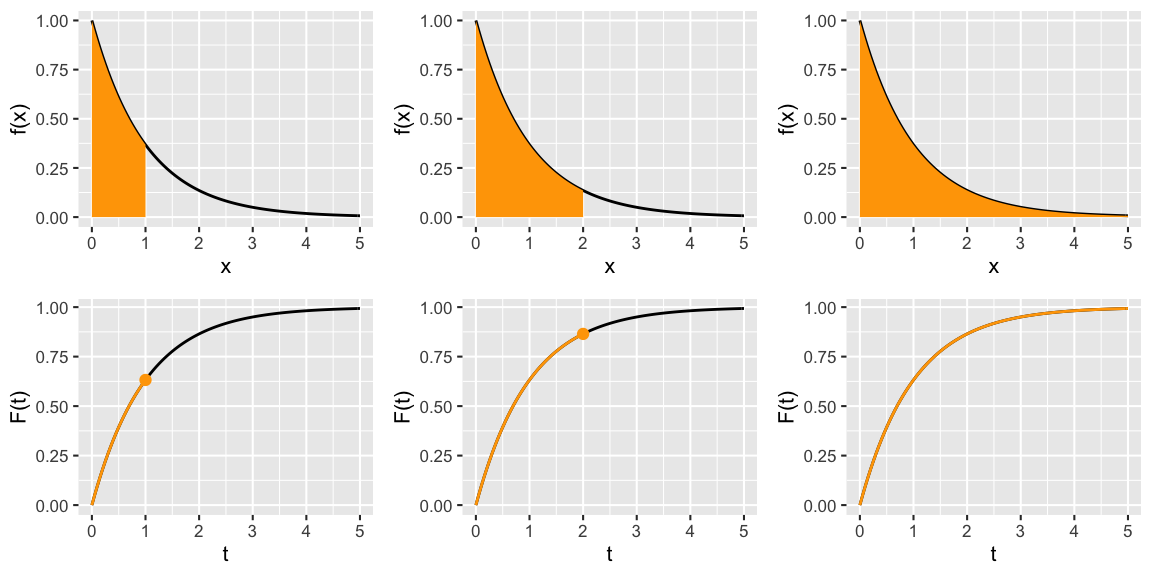
Employees are given a task to do in 1 hour. Let \(X\) be the time (in hours) that it takes an employee to complete the task. \(X\) varies from employee to employee and can be modeled by the pdf
\[f_X (x) = 2x \;\; \text{ for } x \in [0,1]\]

Thus, \(X\) tends to be closer to 1 hour than 0 hours.

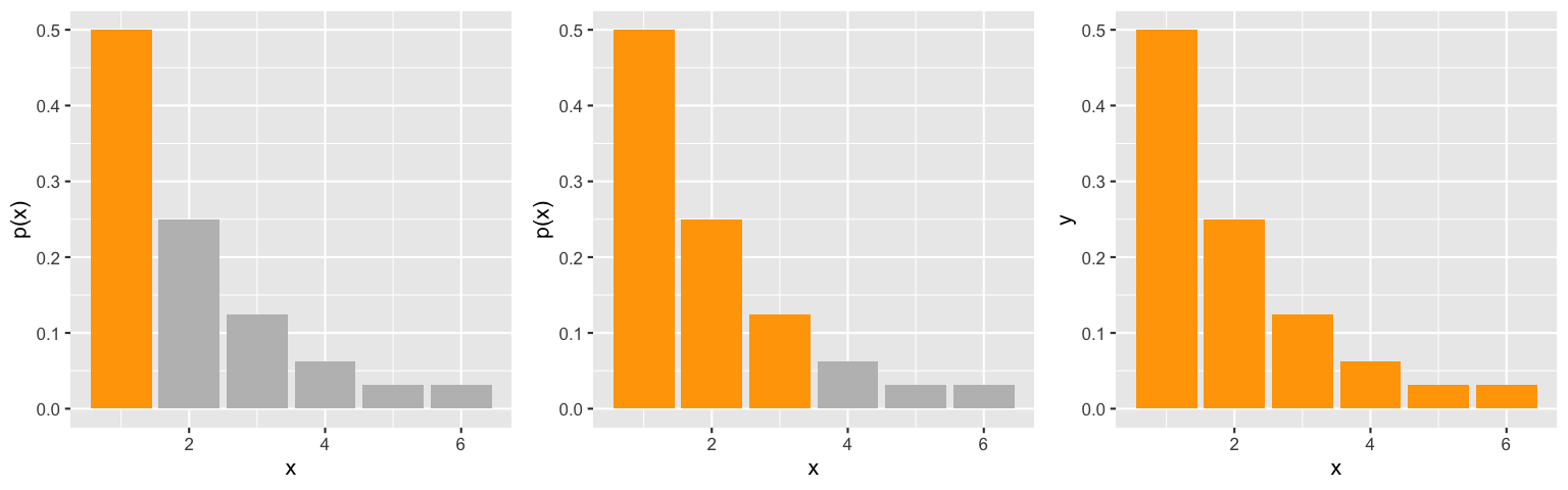
1. Select an employee at random. Calculate and illustrate the following probabilities:
   

2. Derive a function \(F(t) = P(X \le t)\) for \(t \in \mathbb{R}\). Plot \(F(t)\) below:

   

Cumulative Distribution Functions (cdf) & WHY WE CARE!

The cdf of a RV is \[F_X(t) = P(X \le t) \;\; \text{ for } t \in \mathbb{R}\]

Why is cdf \(F_X\) interesting?

1. Like pmfs / pdfs \(p_X\) and \(f_X\), \(F_X\) defines the distribution / model of a RV.

2. For both discrete & continuous RVs, it has an easy & informative interpretation as a probability!

3. It tells us about the rate at which \(X\) accumulates mass/density.

4. It’s the feature of interest in many prob/stat applications.
   • Survival analysis:
     \(F_X(t) = P(\text{survival time } \le t)\)
   • Finite population sampling:
     \(F_X(t) = P(\text{proportion of NE lakes that are dangerously acidic } \le t)\)
     \(F_X(t) = P(\text{proportion of US adults that are unemployed } \le t)\)

CALCULATING A CDF

For continuous RV \(X\) \[F_X(t) = P(X \le t) = \int_{-\infty}^t f_X(x) dx\]

For discrete RV \(X\) \[F_X(t) = P(X \le t) = \sum_{\text{all } x \le t} p_X(x)\]

11.2 Exercises

11.2.1 PART 1

In PART 1 you’ll build CDFs for the continuous and discrete uniform models. We’ll discuss PART 1 as a class before moving on.

1. Suppose that the “The Big Wheel” on The Price Is Right is equally likely to stop at any position on the wheel. Let \[X \sim \text{Unif}(0,360)\] be the angle between the wheel’s final resting place and its starting location. Then \(X\) has pdf \[f_X(x) = \frac{1}{360} \text{ for } x \in [0,360]\;.\]

   
   

   1. To calculate the cdf, \(F_X(t) = P(X \le t)\), we first break up the values \(t \in \mathbb{R}\) into three disjoint pieces: \(t < 0\) (below the support), \(0 \le t \le 360\) (the support), and \(t > 360\) (above the support). For each, derive a formula for \(P(X \le t)\). NOTE: It would help to draw pictures!

      \(t\)	\(P(X \le t)\)	Hint
      \(t < 0\)	\(\hspace{1in}\)	What’s \(P(X \le -10)\)? \(P(X \le -1)\)?
      \(0 \le t \le 360\)		What’s \(P(X \le 100)\)? \(P(X \le 200)\)?
      \(t > 360\)		What’s \(P(X \le 500)\)? \(P(X \le 1000)\)? NOT 0.

   
   

   2. After examining the table, define the cdf: \[F_X(t) = P(X \le t) = \begin{cases} \;\;\;\;\;\;\;\;\;\; & \;\; t < 0 \\ & \;\; 0 \le t < 360 \\ & \;\; t \ge 360 \\ \end{cases}\]

   
   

   3. Finally, plot both the pdf and cdf of \(X\):

      

2. Next, we use our computer’s random number generator to sample a number from \(\{1, 2, 3\}\). Let \(X\) be the chosen number where \(X\) is equally likely to be 1, 2, or 3. Thus \(X\) has a discrete Uniform distribution with pmf \[p_X(x) = 1/3 \;\; \text{ for } x \in \{1,2,3\}\]

   
   

   1. To calculate the cdf, \(F_X(t) = P(X \le t)\), break up the values \(t \in \mathbb{R}\) into disjoint pieces and calculate \(F_X(t)\) for each.

      \(t\)	\(P(X \le t)\)	Hint
      \(t < 1\)		What’s \(P(X \le 0)\)? \(P(X \le -1)\)?
      \(t=1\)
      \(1 < t < 2\)		What’s \(P(X \le 1.5)\)? NOT 0.
      \(t=2\)
      \(2 < t < 3\)		What’s \(P(X \le 2.5)\)? NOT 0.
      \(t=3\)
      \(t > 3\)		What’s \(P(X \le 10)\)? NOT 0.

   
   

   2. After examining the table, define the cdf: \[F_X(t) = P(X \le t) = \begin{cases} \;\;\;\;\;\;\; & \;\; t < 1 \\ & \;\; 1 \le t < 2 \\ & \;\; 2 \le t < 3 \\ & \;\; t \ge 3 \\ \end{cases}\]

   
   

   3. Finally, plot both the pmf and cdf of \(X\):

      

11.2.2 PART 2

In PART 2, you’ll generalize your observations of the Uniform model to CDFs for general RVs.

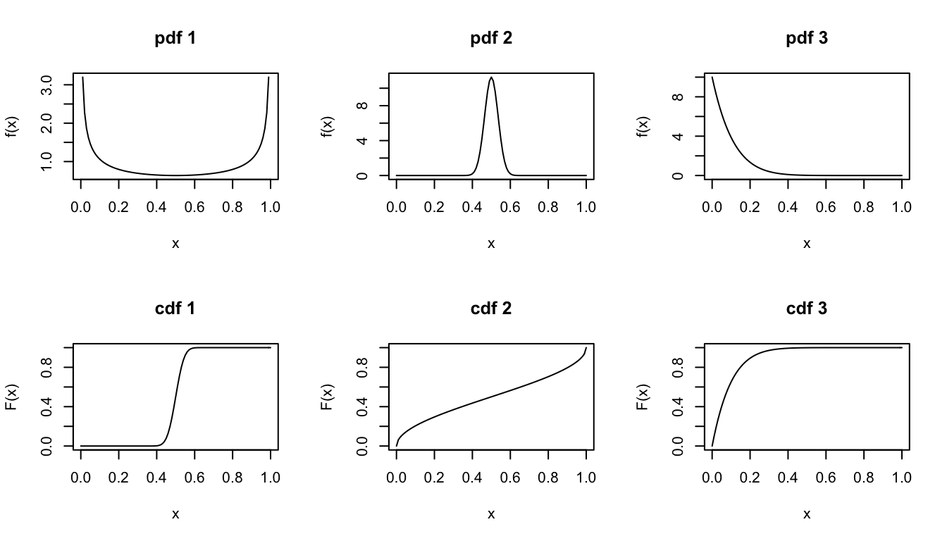
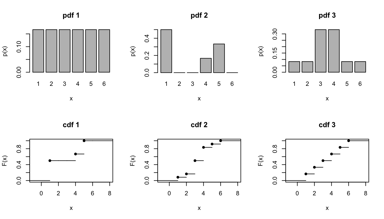
3. Above you’ve explored how cdfs capture the degree to which pdfs accumulate mass/density across \(\mathbb{R}\). Apply these concepts to match the continuous pdfs (top row) with the appropriate continuous cdfs (bottom row).

   

4. Similarly, match the discrete pmfs (top row) to the correct discrete cdf (bottom row).

   

Properties of cdfs

After completing the exercises above, you should see some the cdf properties emerging.

• Limits
  \(F_X(t) = P(X \le t) \to 1\) as \(t \to \infty\)
  \(F_X(t) = P(X \le t) \to 0\) as \(t \to -\infty\)

• Direction
  \(F_X(t)\) is a non-decreasing function between 0 and 1
  Discrete \(X\): \(F_X(t)\) is a right continuous step function
  Continuous \(X\): \(F_X(t)\) is a continuous function

• Shape
  \(F_X(t)\) is steeper in areas of high density/mass and flatter in areas of lower density/mass

11.2.3 PART 3

Above, you explored how to build a CDF from a PDF / PMF. Below, you’ll do the reverse: build a PDF / PMF from a CDF!

5. Consider the following cdf for a continuous RV \(X\): \[F_X(t) = P(X \le t) = \begin{cases} 0 & t < 0 \\ t^4 & 0 \le t < 1 \\ 1 & t \ge 1 \end{cases}\] In pictures:

   

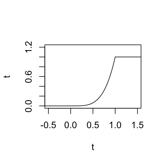
   1. We’ve seen how to derive cdf \(F_X\) from a pdf \(f_X\): \[F_X(t) = P(X \le t) = \int_{-\infty}^tf_X(x)dx\] What about the reverse? Show how to derive pdf \(f_X\) from \(F_X\). Be sure to specify the support for \(f_X\). HINT: Fundamental Theorem of Calculus.

   2. Sketch the pdf \(f_X\).

6. Finally, consider a discrete RV \(X\) with cdf \[F_X(t) = \begin{cases} 0 & t < 0 \\ 0.5 & 0 \le t < 10 \\ 0.7 & 10 \le t < 15 \\ 1 & t \ge 15 \\ \end{cases}\]

   1. Sketch the cdf \(F_X(t)\).

   2. Use the cdf to derive and sketch the pmf \(f_X(x)\). HINTS: Where are the jumps? How big is each jump?

11.3 Summary

For continuous RV \(X\) \[F_X(t) = P(X \le t) = \int_{-\infty}^t f_X(x) dx\]

For discrete RV \(X\) \[F_X(t) = P(X \le t) = \sum_{\text{all } x \le t} p_X(x)\]