24 Sampling distributions: Central Limit Theorem for means
24.1 Discussion
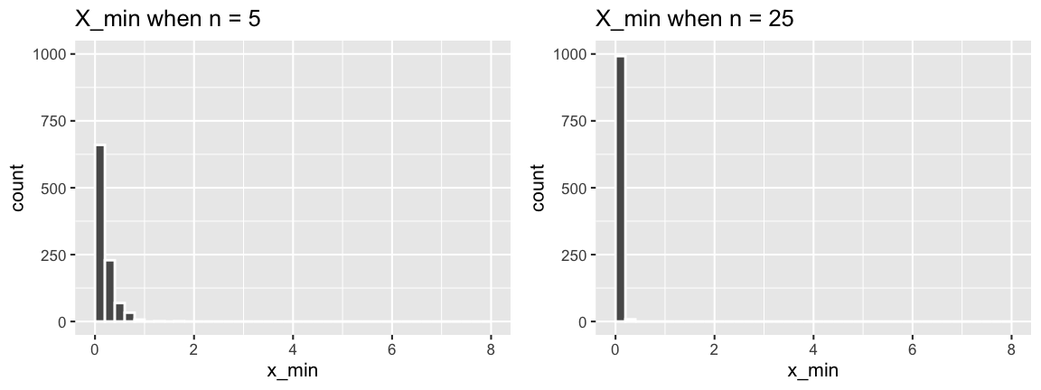
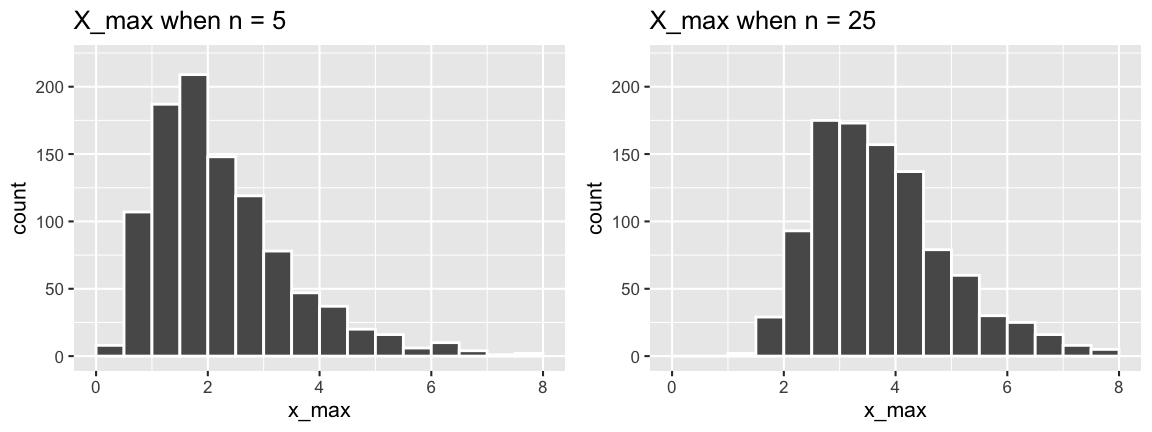
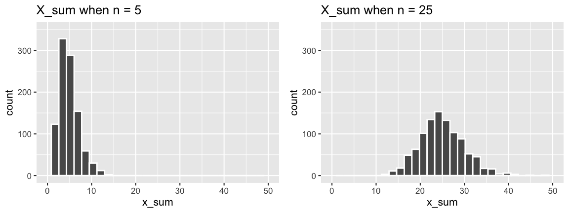
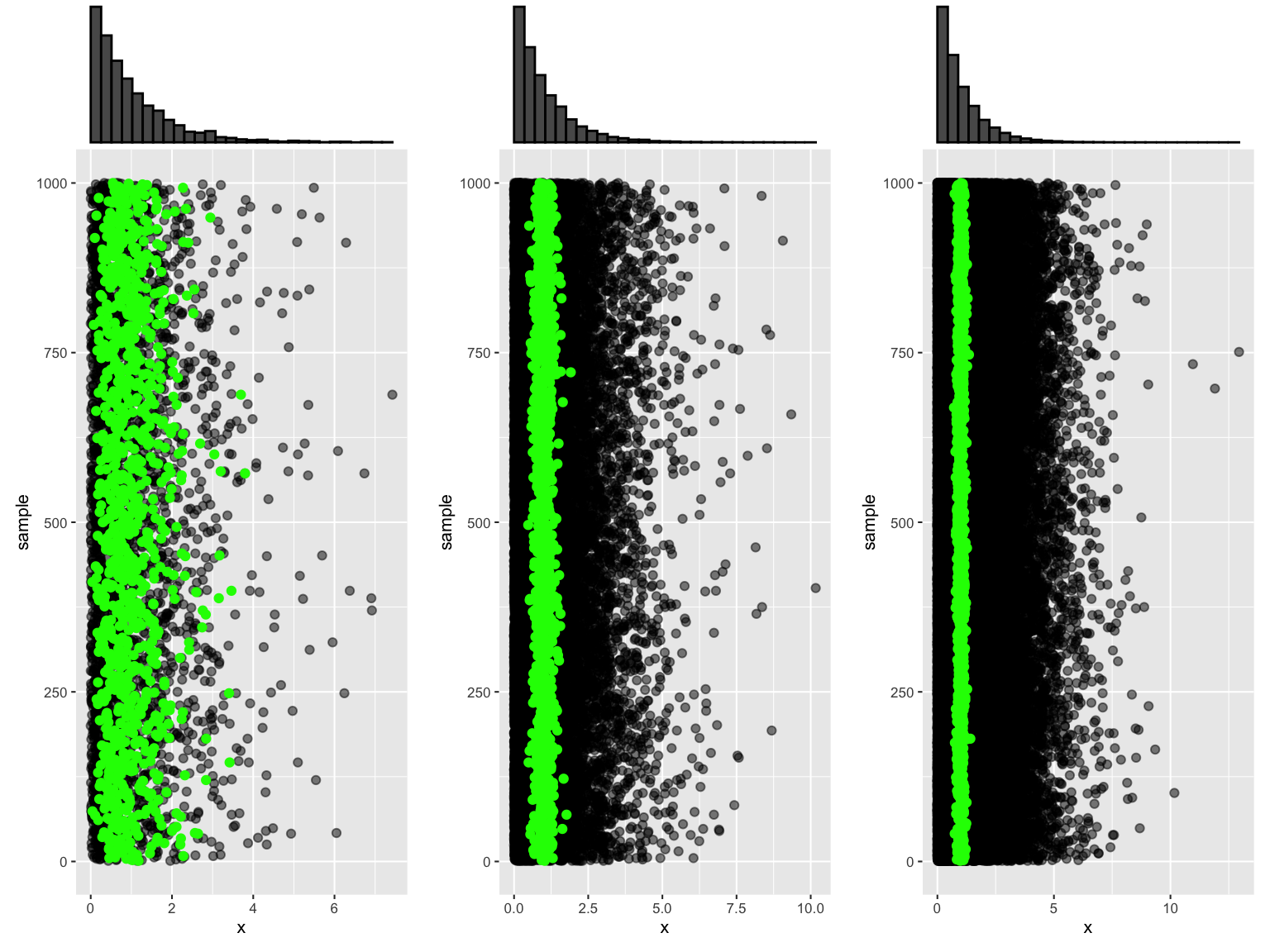
RECALL: Exponential \(X_{min}\), \(X_{max}\), and \(X_{sum}\)
The sampling distributions of \(X_{min}\), \(X_{max}\), and \(X_{sum}\) for an iid sample (\(X_1,...,X_n\)) from Exp(\(\lambda\)) are as follows:
\[\begin{split} X_{min} & \sim Exp(n\lambda) \;\; \text{ with } f_{X_{min}}(x) = (n\lambda)e^{-(n\lambda)x} \;\; \text{ for } x > 0 \\ X_{max} & \text{ has } f_{X_{max}}(x) = n\lambda e^{-\lambda x}\left[1 - e^{-\lambda x}\right]^{n-1} \;\; \text{ for } x > 0 \\ X_{sum} & \sim Gamma(n, \lambda) \;\; \text{ with } f_{X_{sum}}(x) = \frac{\lambda^n}{\Gamma(n)}x^{n-1}e^{-\lambda x} \;\; \text{ for } x > 0 \\ \end{split}\]
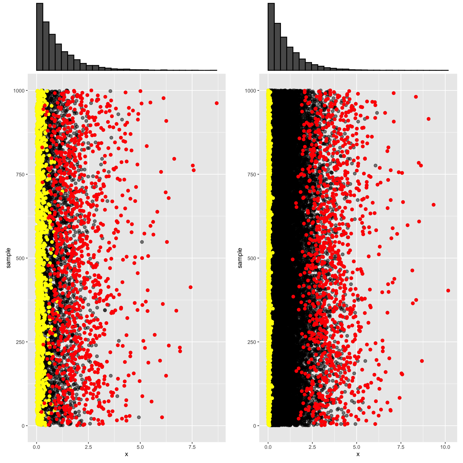
We simulated these sampling distributions under different scenarios, taking 1000 samples of size \(n\) from Exp(1) and recording the \(X_{min}\), \(X_{max}\), and \(X_{sum}\) of each.
EXAMPLE 1: Simulating the sample mean
Similarly, the sample mean
\[\overline{X} = \frac{\sum_{i=1}^nX_i}{n}\]
can vary from sample to sample:
Focusing on just the sample means:

These sample means have the following properties:
## # A tibble: 3 x 4
##       n  mean     sd     var
##   <dbl> <dbl>  <dbl>   <dbl>
## 1     3 0.990 0.572  0.328
## 2    25 1.00  0.201  0.0403
## 3   100 1.00  0.0979 0.00960
Based on these simulation results:
Where are the sampling distributions of \(\overline{X}\) centered? Does this vary depending upon sample size \(n\)? And what does this mean?
How does the variability in the sampling distributions of \(\overline{X}\) depend upon sample size \(n\)? And what does this mean?
Describe the shapes of the sampling distributions of \(\overline{X}\). Does this vary depending upon sample size \(n\)?
CENTRAL LIMIT THEOREM
Let \((X_1, X_2, \ldots, X_n)\) be an iid sample from ANY model (Pois, N, Bin, Exp,…) with \(E(X_i) = \mu\) and \(Var(X_i) = \sigma^2\). Then as sample size \(n \to \infty\) \[\overline{X} \to N\left(\mu, \left(\frac{\sigma}{\sqrt{n}}\right)^2\right)\]
In words:
The value of sample mean \(\overline{X}\) varies from sample to sample, depending on what data we happen to get. BUT as long as the sample size is “big enough”, the different sample means \(\overline{X}\) we could get are (approximately) Normally distributed around the population mean \(\mu\) with decreasing variability as \(n\) increases.
In the words of bunnies
As explained by bunnies & dragons
CLT: WHO CARES?
The CLT is one of the most important theorems in the practice of statistics and data science! If you’ve taken STAT 155, every hypothesis test and confidence interval you explored was built upon this theorem. Why? Well, in practice, we don’t know \(\mu\). Knowing how \(\overline{X}\) behaves allows us to assess how far \(\overline{X}\) might be from \(\mu\) (ie. how much error there is in using \(\overline{X}\) to estimate \(\mu\)).
Examples
- Political polls
- What we want to know:
Trump’s approval rating \(\mu\) amongst all U.S. adults
- What we have:
Trump’s approval rating \(\overline{X}\) in a poll / sample of U.S. adults
- What the CLT gives us:
A sense of the uncertainty in \(\overline{X}\), thus what we can & can’t conclude about \(\mu\).
- What we want to know:
- Scientific studies
- What we want to know:
Effectiveness of a vaccine, as measured by the proportion of people it protects (\(\mu\)), across all people in the world.
- What we have:
Effectiveness of the vaccine, as measured by the proportion of people it protects (\(\overline{X}\)), in a sample of patients.
- What the CLT gives us:
A sense of the uncertainty in \(\overline{X}\), thus what we can & can’t conclude about \(\mu\).
- What we want to know:
- Models
- What we want to know:
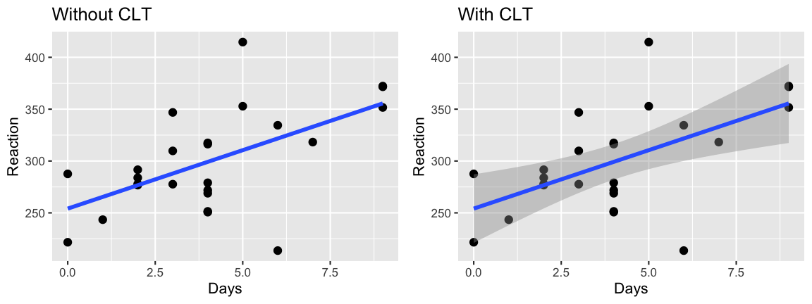
Relationship between reaction time \(Y\) and the number of days of sleep deprivation \(X\) (\(Y = \beta_0 + \beta_1 X\)) across all adults.
- What we have:
Relationship between reaction time \(Y\) and the number of days of sleep deprivation \(X\) (\(Y = b_0 + b_1 X\)) across a sample of adults.
- What the CLT gives us:
A sense of the uncertainty in the sample estimate, thus what we can & can’t conclude about the relationship between \(Y\) and \(X\) in the general population.
- What we want to know:

24.2 Exercises
24.2.1 Background
Properties of the sample mean
Let \((X_1,X_2,...,X_n)\) be an iid sample from ANY model. Thus the \(X_i\) have a common MGF \(M_X(t)\), mean \(\mu\), and variance \(\sigma^2\). Prove that the sample mean \[\overline{X} = \frac{1}{n}\sum_{i=1}^n X_i\] has the following properties:\[\begin{split} E(\overline{X}) & = \mu \\ Var(\overline{X}) & = \frac{\sigma^2}{n} \\ M_{\overline{X}}(t) & = \left[M_X\left(\frac{t}{n}\right)\right]^n \\ \end{split}\]
- Prove these three properties.
- Notice that the sample size \(n\) does NOT impact \(E(\overline{X})\) but DOES impact \(Var(\overline{X})\). Describe this impact: what happens to the variance in \(\overline{X}\) as \(n\) increases?
Explain why your answer to part b makes intuitive sense. For example, suppose there’s a sample of \(n\) students in each classroom at Macalester. You go from room to room to measure the average height in each room:
- Will the variability in classroom averages be more or less than the variability in individual students?
- Suppose each room contains 100 students. Will the variability in the classroom averages be more or less than if each room only had 10 students?
- Will the variability in classroom averages be more or less than the variability in individual students?
Do these results prove the CLT, ie. that so long as \(n\) is large enough, \[\overline{X} \sim N\left(\mu, \left(\frac{\sigma}{\sqrt{n}}\right)^2\right)\]
Solution
.
\[\begin{split} \begin{split} E(\overline{X}) & = E\left(\frac{X_1+X_2+\cdots+X_n}{n} \right) \\ & = \frac{1}{n}E\left(X_1+X_2+\cdots+X_n\right) \\ & = \frac{1}{n}\left(E(X_1) + E(X_2) + \cdots + E(X_n)\right) \\ & = \frac{1}{n}\left(n \mu\right) \\ & = \mu \\ Var(\overline{X}) & = Var\left(\frac{X_1+X_2+\cdots+X_n}{n} \right) \\ & = \frac{1}{n^2}Var\left(X_1+X_2+\cdots+X_n\right) \\ & = \frac{1}{n^2}\left(Var(X_1) + Var(X_2) + \cdots + Var(X_n)\right) \\ & = \frac{1}{n^2}\left(n \sigma^2 \right) \\ & = \frac{\sigma^2}{n} \\ M_{\overline{X}}(t) & = E\left(e^{t\overline{X}}\right) \\ & = E\left(e^{t \frac{X_1+X_2+\cdots+X_n}{n} } \right) \\ & = E\left(e^{\frac{t}{n}X_1}e^{\frac{t}{n}X_2}\cdots e^{\frac{t}{n}X_n}\right) \\ & = E\left(e^{\frac{t}{n}X_1}\right) E\left(e^{\frac{t}{n}X_2}\right) \cdots E\left(e^{\frac{t}{n}X_n}\right) \\ & = \left[M_X\left(\frac{t}{n}\right)\right]^n\\ \end{split}\]- As sample size increases, the variability in the sample mean decreases.
- The bigger the sample size, the more stable the features of the sample. That is, though sample means will vary from sample to sample, they’ll vary less when the samples are large than when they’re small.
- NO!!!!!!! We’ve only proven two properties of the sampling distribution of the sample mean (its trend and variability). Countless models can share this same trend and variability yet, otherwise, behave completely differently. We have yet to prove the CLT.
24.2.2 CLT for the Normal & Exponential
Sampling distribution for a Normal mean: Intuition
Let \((X_1,X_2,...,X_n)\) be an iid sample from a \(N(\mu,\sigma^2)\) model with \(E(X_i) = 0\) and \(Var(X_i) = 1\). To build some intuition for the behavior of sample means \(\overline{X}\) from sample to sample, consider the following simulation results for 1000 samples of size \(n = 4\) (left) and 1000 samples of size \(n = 25\) (right):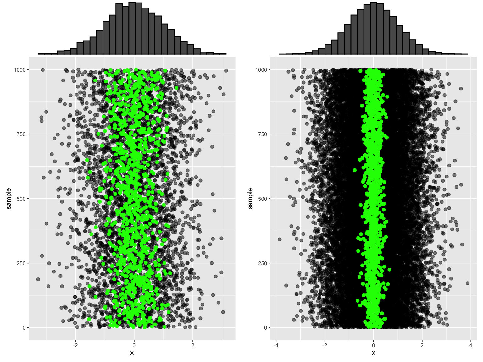
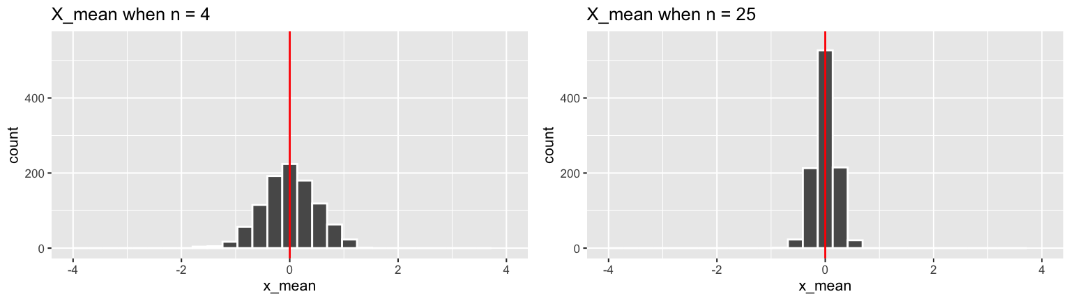
Numerical summaries:
## # A tibble: 2 x 4 ## n mean sd var ## <dbl> <dbl> <dbl> <dbl> ## 1 4 0.0002 0.498 0.248 ## 2 25 -0.002 0.202 0.041- Consider the samples of size \(n = 4\).
- Calculate \(E(\overline{X})\) and \(SD(\overline{X})\), the theoretical expected value and standard deviation of \(\overline{X}\) from sample to sample.
- How close are these theoretical properties to the observed numerical summaries of the simulated \(\overline{X}\) above?
- Calculate \(E(\overline{X})\) and \(SD(\overline{X})\), the theoretical expected value and standard deviation of \(\overline{X}\) from sample to sample.
Repeat for the samples of size \(n = 25\).
You’ve now calculated \(E(\overline{X})\) and \(SD(\overline{X})\). What about the sampling distribution of \(\overline{X}\)? Based on the simulation results, does this appear to be Normal when \(n = 4\)? What about when \(n = 25\)?
Code for the curious
Utilizing the functions from Chapter 22…
# Simulate the samples
set.seed(354)
normal_sim_4 <- sim_data(n = 4, model = "norm")
set.seed(354)
normal_sim_25 <- sim_data(n = 25, model = "norm")

# Plot the 1000 samples
plot_samples(normal_sim_4, plot_mean = TRUE)
plot_samples(normal_sim_25, plot_mean = TRUE)

# Plot the 1000 sample means
ggplot(normal_sim_4, aes(x = x_mean)) +
  geom_histogram(color = "white") +
  labs(title = "X_mean when n = 4") +
  lims(x = c(-4,4), y = c(0,550)) +
  geom_vline(xintercept = 0, color = "red")
ggplot(normal_sim_25, aes(x = x_mean)) +
  geom_histogram(color = "white") +
  labs(title = "X_mean when n = 25") +
  lims(x = c(-4,4), y = c(0,550)) +
  geom_vline(xintercept = 0, color = "red")

# Calculate numerical summaries
normal_sim_4 %>%
  summarize(mean(x_mean), sd(x_mean), var(x_mean))
normal_sim_25 %>%
  summarize(mean(x_mean), sd(x_mean), var(x_mean))
Solution
Let \(\mu = 0\) and \(\sigma = 1\)
- These are very close to the simulated properties!
\(E(\overline{X}) = \mu = 0\), \(SD(\overline{X}) = \sigma / \sqrt{n} = 1 / \sqrt{4} = 0.5\)
- These are very close to the simulated properties!
\(E(\overline{X}) = \mu = 0\), \(SD(\overline{X}) = \sigma / \sqrt{n} = 1 / \sqrt{25} = 0.2\)
- Yes, the sample means appear to vary Normally.
- Consider the samples of size \(n = 4\).
Sampling distribution for a Normal mean: Theory
Now that we have some intuition for the sampling distribution of \(\overline{X}\) for a \(N(\mu,\sigma^2)\) model, let’s establish some theory. Recall that if \(X \sim N(\mu,\sigma^2)\) then\[\begin{split} E(X) & = \mu \\ Var(X) & = \sigma^2 \\ M_X(t) & = e^{\mu t + \sigma^2 t^2 / 2} \\ \end{split}\]
Thus we know from exercise 1 that
\[E(\overline{X}) = \mu \;\; \text{ and } \;\; Var(\overline{X}) = \frac{\sigma^2}{n}\]
However, infinitely many models can share these features. With this in mind, use the MGF to establish the model of \(\overline{X}\). Specify both the name of this model and the parameters upon which it depends.
HINT: \(M_{\overline{X}}(t) = \left[M_X\left(\frac{t}{n}\right)\right]^n\)
Solution
\[\begin{split} M_{\overline{X}}(t) & = \left[M_X\left(\frac{t}{n}\right)\right]^n \\ & = \left[e^{\mu (t/n) + \sigma^2 (t/n)^2 / 2}\right]^n \\ & = \left[e^{(\mu/n)t + (\sigma/n)^2 t^2 / 2}\right]^n \\ & = e^{n(\mu/n)t + n(\sigma/n)^2 t^2 / 2} \\ & = e^{\mu t + (\sigma/\sqrt{n})^2 t^2 / 2} \\ \end{split}\]
This is the MGF of a \(N(\mu, (\sigma/\sqrt{n})^2)\) model. Thus
\[\overline{X} \sim N\left(\mu, \left(\frac{\sigma}{\sqrt{n}}\right)^2\right)\]
Sampling distribution for an Exponential mean
OK! You showed that the sample mean \(\overline{X}\) of a Normal sample is itself Normal! What about the sample mean \(\overline{X}\) of an Exponential sample? You built some intuition for the sampling distribution of \(\overline{X}\) for an \(Exp(\lambda)\) model above. In the setting with \(\lambda = 1\):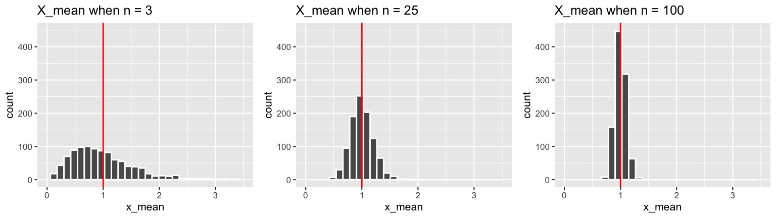
Now let’s establish some theory. Let \((X_1,X_2,...,X_n)\) be an iid sample from an \(Exp(\lambda)\) with
\[\begin{split} \mu & = E(X) = \frac{1}{\lambda} \\ \sigma^2 & = Var(X) = \frac{1}{\lambda^2} \\ M_X(t) & = \frac{\lambda}{\lambda - t} \\ \end{split}\] Thus we know from earlier work that the sample mean has properties
\[E(\overline{X}) = \mu = \frac{1}{\lambda} \;\; \text{ and } \;\; Var(\overline{X}) = \frac{\sigma^2}{n} = \frac{1}{n\lambda^2}\]- Again, the expected value and variance are merely two features of the sampling distribution. To this end, specify the MGF of \(\overline{X}\) and use this to specify the model / sampling distribution of \(\overline{X}\). HINT: If \(Y \sim Gamma(s,r)\), then \(M_Y(t) = \left(\frac{r}{r-t}\right)^s\) for \(t < r\).
Based on your answer to a, can you say that the sampling distribution of an Exponential mean \(\overline{X}\) is exactly Normal?
What does the CLT guarantee about the sampling distribution of an Exponential mean \(\overline{X}\)? As \(n \to \infty\), \[\overline{X} \to ???\]
Are these results consistent with what you saw in the simulations above?
Solution
\(\overline{X} \sim Gamma(n, n\lambda)\) since:
\[\begin{split} M_{\overline{X}}(t) & = \left[M_X\left(\frac{t}{n}\right)\right]^n \\ & = \left[\frac{\lambda}{\lambda - t/n}\right]^n \\ & = \left[\frac{n\lambda}{n\lambda - t}\right]^n \\ \end{split}\]- Nope. It’s Gamma.
As \(n \to \infty\), the sampling distribution of \(\overline{X}\) approaches
\[N\left(\frac{1}{\lambda}, \frac{1}{n\lambda^2} \right)\]Yes.
- Again, the expected value and variance are merely two features of the sampling distribution. To this end, specify the MGF of \(\overline{X}\) and use this to specify the model / sampling distribution of \(\overline{X}\). HINT: If \(Y \sim Gamma(s,r)\), then \(M_Y(t) = \left(\frac{r}{r-t}\right)^s\) for \(t < r\).
24.2.3 USE the CLT
Let \(\pi \in [0,1]\) be Trump’s current approval rating. To estimate \(\pi\), pollsters plan to poll \(n\) Americans and record \((X_1,X_2,...,X_n)\) where \(X_i = 1\) if person \(i\) approves of Trump and 0 otherwise. Thus \[(X_1,X_2,...,X_n) \text{ are iid } Bin(1, \pi)\] with \[\mu = E(X_i) = \pi \;\; \text{ and } \;\; \sigma^2 = Var(X_i) = \pi(1-\pi)\]
Further, the proportion of the sample that approve of Trump is simply the sample mean: \[\overline{X} = \frac{\text{number that approve}}{\text{number polled}} = \frac{\sum_{i=1}^n X_i}{n}\]
Sampling Distribution of a poll result
Poll results can vary from sample to sample. With this in mind, so long as the sample size \(n\) is “big enough”, what does the Central Limit Theorem guarantee about the sampling distribution of \(\overline{X}\)? \[\overline{X} \sim N(???,???)\]
Solution
\[\overline{X} \sim N\left(\pi, \frac{\pi(1-\pi)}{n}\right) = N\left(\pi, \left(\sqrt{\frac{\pi(1-\pi)}{n}}\right)^2\right)\]
- Hypotheticals
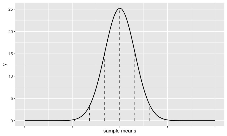
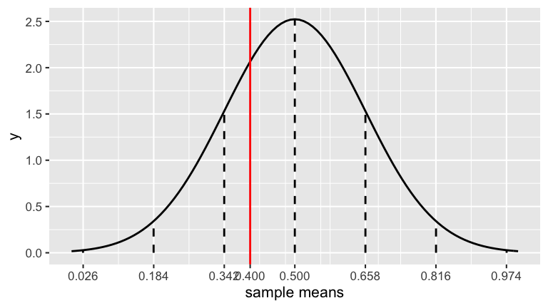
A Trump campaign aide claims that Trump’s approval rating is 50% (ie. that \(\pi = 0.5\)). To test this claim, a pollster conducts a poll of \(n=1000\) people.- Assume the aide’s claim were true. Under this assumption, what kinds of polling results would we expect? To this end, plug \(\pi = 0.5\) and \(n = 1000\) to the CLT from the exercise above to specify the sampling distribution of \(\overline{X}\) in this scenario.
The sampling distribution of \(\overline{X}\) is drawn below. Use the 68-95-99.7 Rule to mark the scale of the x-axis at each vertical line.
Solution
\[\overline{X} \sim N\left(0.5, \left(\sqrt{\frac{0.5(1-0.5)}{1000}}\right)^2\right) = \sim N\left(0.5, \left(\sqrt{0.00025}\right)^2\right)\]
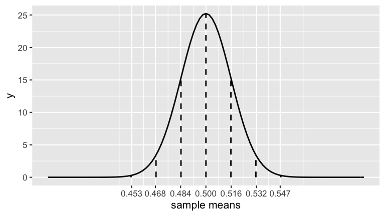
- Assume the aide’s claim were true. Under this assumption, what kinds of polling results would we expect? To this end, plug \(\pi = 0.5\) and \(n = 1000\) to the CLT from the exercise above to specify the sampling distribution of \(\overline{X}\) in this scenario.
Poll results
Upon completing the poll of 1000 Americans, 400 supported Trump. Thus we estimate that Trump has a 40% approval rating: \[\overline{X} = 0.4\]- Mark \(\overline{X}\) on the plot above.
- Comment on where this poll result falls along the scale of poll results we might expect if the aide’s claim that \(\pi = 0.5\) were true.
Using the 68-95-99.7 Rule and the plot above, what can we say about the probability of getting a poll result of 40% approval or even lower (\(\overline{X} \le 0.4\)) IF the aide’s claim were true?
- less than 0.0015
- less than 0.003
- between 0.0015 & 0.025
- between 0.025 & 0.16
- greater than 0.16
- less than 0.0015
BONUS: What’s the probability calculation in part c called in statistics?
Solution
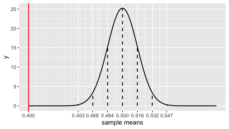
the observed poll result of 0.4 is much smaller than we’d expect if the aide’s claim were true
less than 0.0015 – it’s more than 3 s.d. below the mean
- p-value!!!
- Mark \(\overline{X}\) on the plot above.
Margin of error
When the pollster reported these poll results, they did so with a “margin of error” of \(\pm 3\) percentage points. To understand where this comes from, recall that the 68-95-99.7 Rule guarantees that 95% of samples will have sample means \(\overline{X}\) that are within 2 standard deviations of the population mean. Under Trump’s claim that \(\pi = 0.5\):- What is the range of the middle 95% of potential sample means? (Give an interval.)
- What is the numerical distance between the center and endpoints of this interval?
Solution
\(0.5 \pm 2*\sqrt{\frac{0.5(1-0.5)}{1000}} \approx 0.5 \pm 2*0.016 = (0.468, 0.532)\)
- 0.532 - 0.5 = 0.032…roughly 3 percentage points!!
- What is the range of the middle 95% of potential sample means? (Give an interval.)
Repeat
Suppose that instead, we observed that 4 out of 10 people approved of Trump. Would this be enough evidence to disprove the claim that \(\pi = 0.5\)? Support your answer with some math!
Solution
Nope.
\[\overline{X} \sim N\left(0.5, \left(\sqrt{\frac{0.5(1-0.5)}{10}}\right)^2\right) \approx \sim N\left(0.5, 0.16^2\right)\]
Thus the observed poll of \(\overline{X} = 0.4\) is within 1 s.d. of 0.5 (not convincingly far from the claimed value):
24.2.4 PROVE the CLT!!!
We’ve been using the CLT. Now we’ll prove it. We’ll do this for the following special case, but the general theorem follows directly by properties of linear transformations. Specifically, assume that \((X_1, X_2, \ldots, X_n)\) is an iid from ANY model (Pois, N, Bin, Exp,…) with common MGF \(M_X(t)\), \(\mu = E(X) = 0\), and \(\sigma^2 = Var(X) = 1\). Then the Central Limit Theorem in this setting states that
\[\overline{X} \to N\left(0, \frac{1}{n}\right)\]
as \(n \to \infty\). You’ll prove this in four steps:
- Step 1: Approximate the MGF of \(X\)
- Step 2: Approximate the MGF of the standardized sample mean \(\overline{X}\)
- Step 3: Identify the limiting model of the standardized \(\overline{X}\)
- Step 4: Unstandardize to identify the limiting model of \(\overline{X}\)
Step 1: Approximate the MGF of \(X\)
Since we aren’t making assumptions about the population model, we don’t have a formula for \(M_X(t)\). However, Taylor’s theorem guarantees that \[M_X(t) \approx M_X(0) + M_X^{(1)}(0)t + \frac{1}{2}M_X^{(2)}(0)t^2 + \text{ remainder }\] Use the properties of \(X\) and MGFs with Taylor’s theorem to prove that \[M_X(t) \approx 1 + \frac{1}{2}t^2\]
Solution
By the definition of MGFs:
\[\begin{split} M_X(t) & = E(e^{tX}) \\ M_X(0) & = E(e^{0*X}) = E(1) = 1 \\ M_X^{(1)}(0) & = E(X) = 0 \\ M_X^{(2)}(0) & = E(X^2) = Var(X) - [E(X)]^2 = 1 \\ \end{split}\]
Thus
\[M_X(t) \approx M_X(0) + M_X^{(1)}(0)t + \frac{1}{2}M_X^{(2)}(0)t^2 = 1 + 0*t + \frac{1}{2}*1*t^2 = 1 + \frac{1}{2}t^2\]
Step 2: Approximate the MGF of the standardized sample mean \(\overline{X}\)
Define the standardized sample mean of \(n\) objects as \[Y_n = \frac{\overline{X} - E(\overline{X})}{SD(\overline{X})} = \sqrt{n} \overline{X}\] Prove that the standardized sample mean has the following MGF: \[M_{Y_n}(t) \approx \left[1 + \frac{t^2/2}{n}\right]^n\]
Solution
\[\begin{split} M_{Y_n}(t) & = E(e^{tY_n}) \;\;\; \text{ (by def of MGF)}\\ & = E(e^{t\sqrt{n}\overline{X}}) \;\;\; \text{ (by def of $Y_n$)} \\ & = E(e^{(t\sqrt{n})\overline{X}}) \\ & = M_{\overline{X}}(t\sqrt{n}) \;\;\; \text{ (by def of MGF)} \\ & = \left[M_X(t\sqrt{n})\right]^n \;\;\; \text{ (by Example 1)}\\ & \approx \left[1 + \frac{1}{2}(t\sqrt{n})^2\right]^n \;\;\; \text{ (by step 1)}\\ & = \left[1 + \frac{t^2/2}{n}\right]^n \\ \end{split}\]
- Step 3: Identify the limiting model of the standardized \(\overline{X}\)
Prove that as sample size \(n\) increases, the MGF of the standardized mean \(Y_n\) converges to the MGF of the standardized Normal, thus: \[Y_n \to N(0, 1^2)\] HINTS: You can use the fact that \[\left(1 + \frac{x}{n}\right)^n \to e^x \;\; \text{ as } n \to \infty\] Further, recall that if \(X \sim N(\mu, \sigma^2)\), then \(M_X(t) = e^{\mu t + \sigma^2 t^2 / 2}\).
As \(n \to \infty\), \[M_{Y_n}(t) \approx \left[1 + \frac{t^2/2}{n}\right]^n \to e^{t^2} = e^{0*t + 1^2*t^2/2}\] which is the MGF of a N(0,1) model!
Step 4: Unstandardize to identify the limiting model of \(\overline{X}\)
Prove that as \(n\to \infty\), the Central Limit Theorem holds!!! \[\overline{X} \to N\left(0, \frac{1}{n}\right)\]
Solution
\(\overline{X} = Y_n/\sqrt{n}\), thus
\[\begin{split} M_{\overline{X}}(t) & = E(e^{t\overline{X}}) \\ & = E(e^{t/\sqrt{n} Y_n) \\ & = M_{Y_n}(t/\sqrt{n}) \\ & \to e^{(t/\sqrt{n})^2} \;\; \text{(the MGF of $N(0,(1/\sqrt{n})^2)$)} \\ \end{split}\]
24.3 Congratulations!!
You proved one of the most exciting and well known theorems ever in the history of all theorems!