4 Monte Carlo simulation
RECOMMENDED READING
B & H Chapters 1.6 - 1.7.
4.1 Discussion
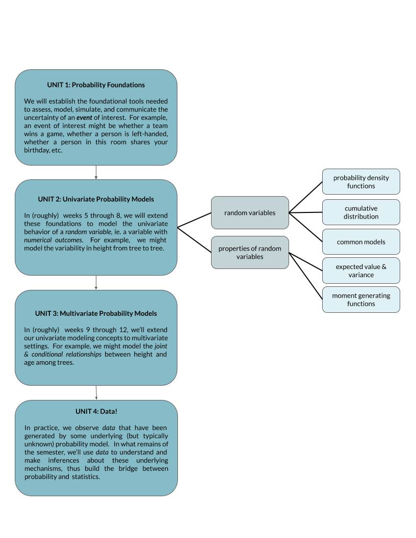
Monte Carlo simulation is a critical tool that we’ll use throughout the semester to explore and approximate uncertainty. The basic idea is similar to using a physical coin to understand its fairness (ie. the probability of observing Heads):
- Flip the coin over and over and over.
- Record the proportion of Heads in these sample flips.
- The more times we flip the coin, the better these sample proportions approximate the “true” fairness of the coin.
The main difference is that in a Monte Carlo simulation, we use a computer to do the heavy lifting!
History
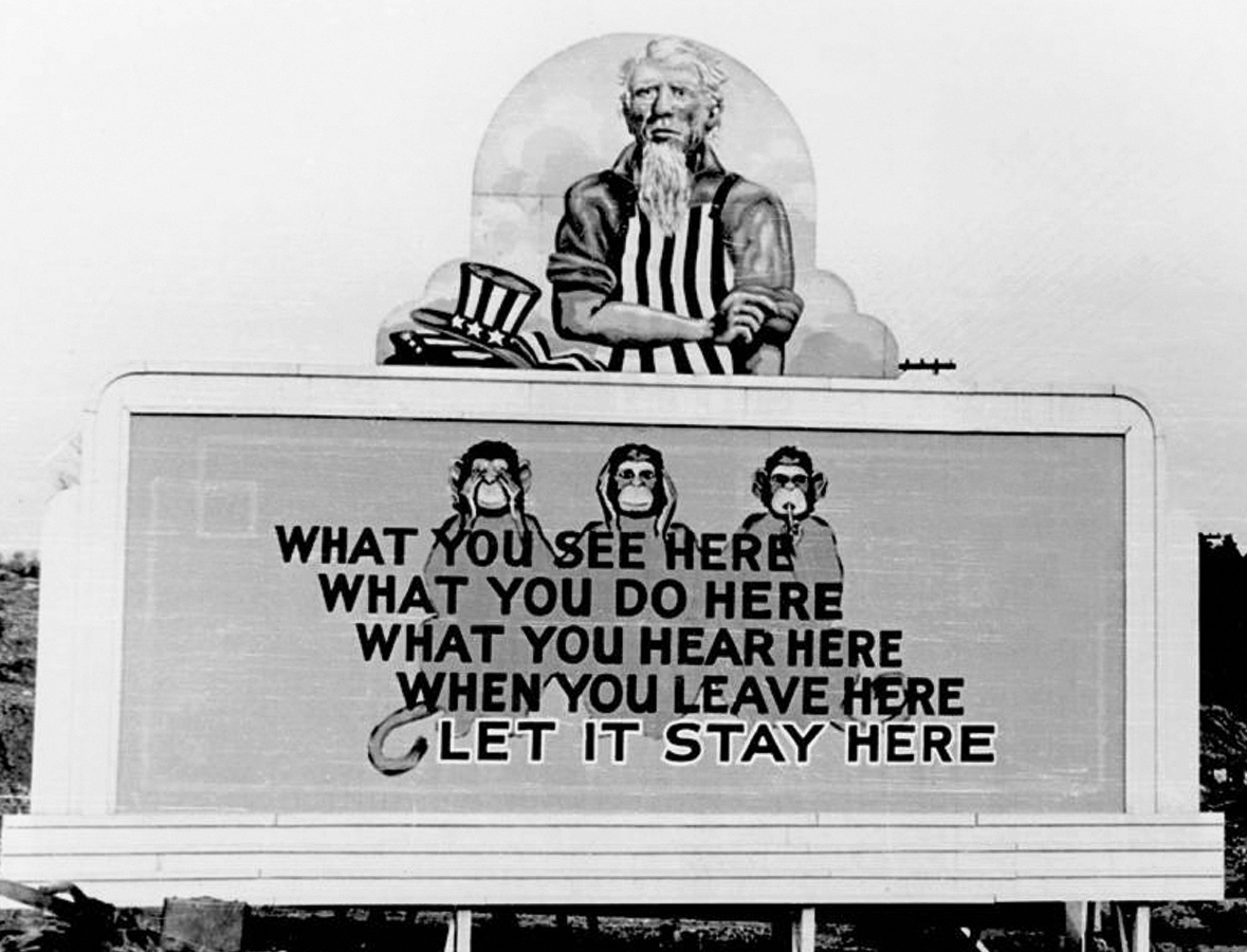
“Monte Carlo” was the code name used by Stanislav Ulam, John von Neumann, et al for their top secret nuclear weapons project at the Los Alamos National Laboratory in the 1940’s2
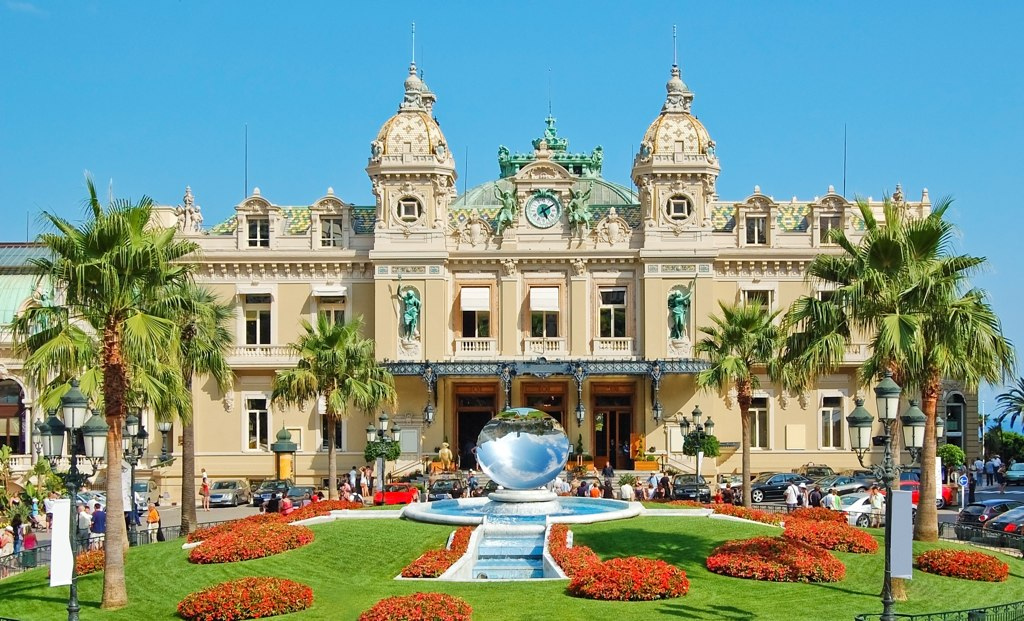
The code name was inspired by the opulent Monte Carlo casino in the equally opulent Principality of Monaco on the French Riviera.3 (See other excellent code names.).
4.2 Exercises
There are 10 marbles in an urn: 4 green (\(G\)), 5 red (\(R\)), and 1 white (\(W\)). Thus if you pick a marble at random:
\[P(G) = 0.4, \; P(R) = 0.5, \; P(W) = 0.1\]
We’ll run a Monte Carlo simulation study in RStudio to connect these probabilities to what we’d actually observe in repeated observations of this experiment. In doing so:
- Open the Rmd (Rmarkdown) template on Moodle.
- Run the provided code one chunk at a time, taking care to identify what each line achieves!
- You’re encouraged to take notes in Rmarkdown, but do whatever is most comfortable to you.
- Some code chunks have blanks for you to fill in. These include an
eval = FALSEstatement to indicate that they should not yet be evaluated – if they were, they would produce errors. Once you’ve filled in the blanks and your code is working, either eliminate theeval = FALSEstatement or change it toeval = TRUE.
Load packages
Review
sample_n()
Set up the marbles.# Create a data frame of the marble colors marbles <- data.frame(color = c("G","R","W")) marbles ## color ## 1 G ## 2 R ## 3 WUse
sample_n()to sample 3 marbles with replacement and 3 marbles without replacement:Run the following chunk multiple times. How does the
weightargument impact the results?
- Run the marble experiment 100 times
Fill in the blanks to run the marble experiment (with the original probabilities) 100 times. Store the results in a data frame named
run_100.Count up the number of times you picked each color.
Plot the number of times you picked each color.
Check out the table from part b. How close are the observed color proportions to the theoretical probabilities, \(P(G),P(R),P(W)\)?
Solution
- Run the marble experiment 10,000 times
Repeat the above exercise, this time running the experiment 10,000 times (not 100 times). Now how close are the observed color proportions to their theoretical probabilities?
Reproducibility
Sampling is inherently random. Your results can differ every time you repeat the experiment. But it’s important to be able to reproduce your results (we’ll chat about this as a class). To this end, you can set the random number generating seed to a positive integer, here 354. Run the following code chunk multiple times. You should get the same answer every time AND the same answer as your neighbor!# Set the random number generating seed set.seed(354) # Run the marble experiment 10000 times final_run <- sample_n(marbles, size = 10000, replace = TRUE, weight = c(0.4,0.5,0.1)) # Tabulate the observed color final_run %>% ___(___) %>% ___("row")
Solution
# Set the random number generating seed
set.seed(354)

# Run the marble experiment 10000 times
final_run <- sample_n(marbles, size = 10000, replace = TRUE, weight = c(0.4,0.5,0.1))

# Tabulate the observed color
final_run %>%
  tabyl(color) %>%
  adorn_totals("row")
##  color     n percent
##      G  4041  0.4041
##      R  4931  0.4931
##      W  1028  0.1028
##  Total 10000  1.0000
- Conditional probability
A pig comes along and eats one of your marbles. Unfortunately, you weren’t close by and so could only make out that the marble was not red. In light of this information, the probability that the pig ate a green marble jumps from \(P(G) = 0.4\) to \[P(G|R^c) = 0.8\]
Let’s support this calculation using thefinal_runsimulation.In general, conditional information restricts the sample size. In this case, we can use the
filter()function to restrict the simulation results to only those that don’t have a red marble. We store this new dataset asnot_red:Note:
!== “not equal to”Calculate the proportion of each color remaining in the
not_redmarbles. Does this (approximately) match the 0.8 calculation?
- Try again
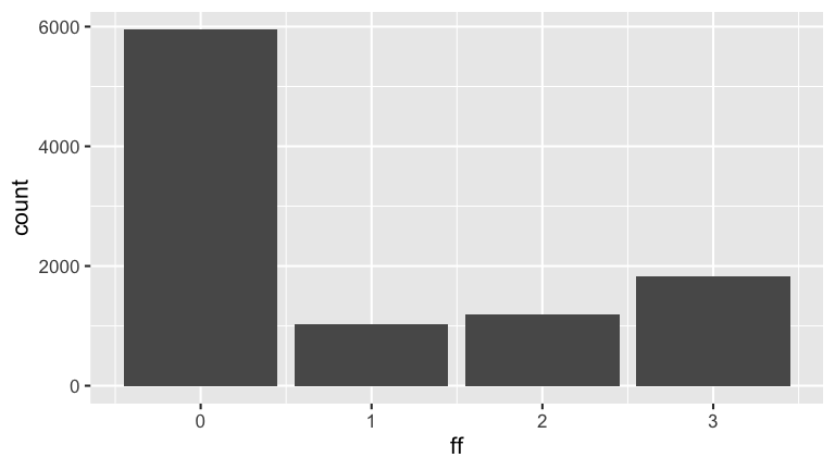
Suppose that 60% of Mac students have seen 0 Fast & Furious films, 10% have seen 1, 12% have seen 2, and 18% have seen 3.- Pick a Mac student at random. Simulate the probabilities that they’ve seen 0, 1, 2, or 3 F&F films. Summarize these with a visualization and table.
- Use this simulation to approximate the conditional probability that a student has seen 3 F&F films if we learn that they’ve seen more than 0.
Solution
4.3 Extra practice in a more complicated setting
If you’ve finished and absorbed the exercises above, keep going! Recall our study in the previous activity. A new friend tells you that they have 2 children. To greatly oversimplify things, we’ll assume binary gender identities for both children: boy or girl. Define the following events:
- \(A\) = both children are boys
- \(B\) = at least one child is a boy
- \(C\) = at least one child is a boy that was born in the morning
- \(D\) = the eldest child is a boy that was born in the morning
We showed that \(P(A) < P(A|B) < P(A|C) < P(A|D)\). Most people find this surprising. In such scenarios we can support and gain insight into our calculations using Monte Carlo simulation.
Supporting our results with simulation
We’ll start as simply as possible, focusing only on the gender identities of the two children. To this end, we’ll simulate this information for 10,000 pairs of siblings. NOTE: There are many ways to do this. We’ll start with an approach that matches the logical steps in our thinking, though isn’t very efficient. If time allows, you can explore a more computationally efficient approach at the end of the activity.# Set up the sample space gender_id <- data.frame(id = c("b","g")) # Set the random number seed set.seed(354) # Simulate the gender_id of child 1 gender_id_1 <- sample_n(gender_id, size = 10000, replace = TRUE) # Simulate the gender_id of child 2 gender_id_2 <- sample_n(gender_id, size = 10000, replace = TRUE) # Store the simulated pairs in a data frame children <- data.frame(gender_id_1 = gender_id_1$id, gender_id_2 = gender_id_2$id) # Check out the first 3 pairs head(children, 3) ## gender_id_1 gender_id_2 ## 1 g b ## 2 b g ## 3 b bUse info from the following table to confirm that our calculation that \(P(A) = 0.25\) was reasonable. Take note of how
tabyl()can be used to summarize two variables.Suppose you learn that at least 1 child is a boy (\(B\)). Restrict the simulation data to only the results that match this info. NOTE:
|is the RStudio equivalent of “or” or \(\cup\).Construct a table of these results to confirm your earlier calculation that \(P(A|B) = 1/3\) was reasonable.
Solution
# Tabulate all combinations of birth gender_id children %>% tabyl(gender_id_1, gender_id_2) %>% adorn_totals(c("row","col")) ## gender_id_1 b g Total ## b 2470 2522 4992 ## g 2531 2477 5008 ## Total 5001 4999 10000 2470 / 10000 ## [1] 0.247 # Keep only the cases that match information B info_B <- children %>% filter(gender_id_1 == "b" | gender_id_2 == "b") # Check out the results dim(info_B) ## [1] 7523 2 head(info_B) ## gender_id_1 gender_id_2 ## 1 g b ## 2 b g ## 3 b b ## 4 b b ## 5 b g ## 6 b g info_B %>% tabyl(gender_id_1, gender_id_2) %>% adorn_totals(c("row","col")) ## gender_id_1 b g Total ## b 2470 2522 4992 ## g 2531 0 2531 ## Total 5001 2522 7523 2470/7523 ## [1] 0.3283265
- Incorporating time of day
Next, let’s incorporate the birth time of day into our analysis.For each of the 10,000 pairs of simulated children, simulate & store a birth time of day (\(m\) = morning or \(n\) = night). NOTE: we must use a different random number seed than when we generated
gender_id_1andgender_id_2or else the time variables would be exactly the same as the gender_id variables, just with different numbers!# Set up the sample space of birth time of day time_of_day <- data.frame(time = c("m", "n")) # Set the random number seed set.seed(27) # Simulate the birth time of child 1 time_of_day_1 <- ___ # Simulate the birth time of child 2 time_of_day_2 <- ___ # Incorporate time into data frame using mutate() children <- children %>% mutate(time_of_day_1, time_of_day_2) # Check out the first 6 pairs head(children)- What does the
mutate()function do in part a?
Suppose you learn that at least 1 child was a boy born in the morning (\(C\)). Restrict the simulation data to only the results that match this info and subsequently construct a table from which you can confirm that your earlier calculation that \(P(A|C) = 3/7 \approx 0.429\) is reasonable. NOTE:
&is the RStudio equivalent of “and” or \(\cap\).Similarly, simulate \(P(A|D)\) which we earlier calculated to be 0.5.
Solutions
# Set up the sample space of birth time of day
time_of_day <- data.frame(time = c("m", "n"))

# Set the random number seed
set.seed(27)

# Simulate the birth time of child 1
time_of_day_1 <- sample_n(time_of_day, size = 10000, replace = TRUE)

# Simulate the birth time of child 2
time_of_day_2 <- sample_n(time_of_day, size = 10000, replace = TRUE)

# Incorporate time into data frame using mutate()
children <- children %>%
    mutate(time_of_day_1 = time_of_day_1$time, time_of_day_2 = time_of_day_2$time)

# Check out the first 6 pairs
head(children)
##   gender_id_1 gender_id_2 time_of_day_1 time_of_day_2
## 1           g           b             m             n
## 2           b           g             n             n
## 3           b           b             n             m
## 4           b           b             m             n
## 5           b           g             n             n
## 6           b           g             m             n

info_C <- children %>%
  filter((gender_id_1 == "b" & time_of_day_1 == "m") | (gender_id_2 == "b" & time_of_day_2 == "m"))

info_C %>%
  tabyl(gender_id_1, gender_id_2) %>%
  adorn_totals(c("row","col"))
##  gender_id_1    b    g Total
##            b 1862 1261  3123
##            g 1297    0  1297
##        Total 3159 1261  4420

1862/4420
## [1] 0.421267

info_D <- children %>%
  filter(gender_id_1 == "b" & time_of_day_1 == "m")

info_D %>%
  tabyl(gender_id_1, gender_id_2) %>%
  adorn_totals(c("row","col"))
##  gender_id_1    b    g Total
##            b 1201 1261  2462
##            g    0    0     0
##        Total 1201 1261  2462

1201/2462
## [1] 0.4878148
Building intuition
So long as you set the seed, your Monte Carlo approximations should match those below. Comment on the trend in the denominators and explain the significance of this trend.\[\begin{split} P(A) & \approx \frac{2470}{10000} = 0.247 \\ P(A|B) & \approx \frac{2470}{7523} \approx 0.328 \\ P(A|C) & \approx \frac{1862}{4420} \approx 0.421 \\ P(A|D) & \approx \frac{1201}{2462} \approx 0.488 \\ \end{split}\]
Even more extra: a more efficient simulation
Above, we simulated the simulated separate vectors ofgender_idandtime_of_dayfor each child, then combined these into a data frame. A more efficient approach is to first define the sample space of all possible combinations ofgender_id&time_of_dayfor a pair of children, then sample from these.Confirm that the following produces a valid sample space of all possible combinations of
gender_id&time_of_dayfor a pair of children.We can sample rows from the
sample_spaceusingsample_n()!# Set the seed set.seed(354) # Sample 100000 scenarios from sample_space child_sim <- sample_n(sample_space, size = 10000, replace = TRUE) # Check it out dim(child_sim) ## [1] 10000 4 head(child_sim) ## gender_id_1 time_of_day_1 gender_id_2 time_of_day_2 ## 1 g m g m ## 2 b n b n ## 3 b m g m ## 4 b n b m ## 5 b n g n ## 6 b m b nUse
child_simas you usedchildrenabove to support your calculations of \(P(A)\) and \(P(A|B)\).
Solution
child_sim %>%
  tabyl(gender_id_1, gender_id_2) %>%
  adorn_totals(c("row","col"))
##  gender_id_1    b    g Total
##            b 2489 2503  4992
##            g 2508 2500  5008
##        Total 4997 5003 10000

2489/10000
## [1] 0.2489

child_sim %>%
  filter(gender_id_1 == "b" | gender_id_2 == "b") %>%
  tabyl(gender_id_1, gender_id_2) %>%
  adorn_totals(c("row","col"))
##  gender_id_1    b    g Total
##            b 2489 2503  4992
##            g 2508    0  2508
##        Total 4997 2503  7500

2489/7500
## [1] 0.3318667
- Recommended note taking
To help out your future self, provide a summary of what the following functions do and how they work:head(),sample_n(),set.seed(),tabyl(),filter(),mutate(),ggplot()
A billboard at uranium processing plant in Oak Ridge, TN, a sister site of Los Alamos. (https://simple.wikipedia.org/wiki/Manhattan_Project)↩
The Monte Carlo Casino in Monaco. image: https://www.flickr.com/photos/nat507/16530961901↩