14 Functions of Random Variables
14.1 Discussion
Functions of random variables are random variables!
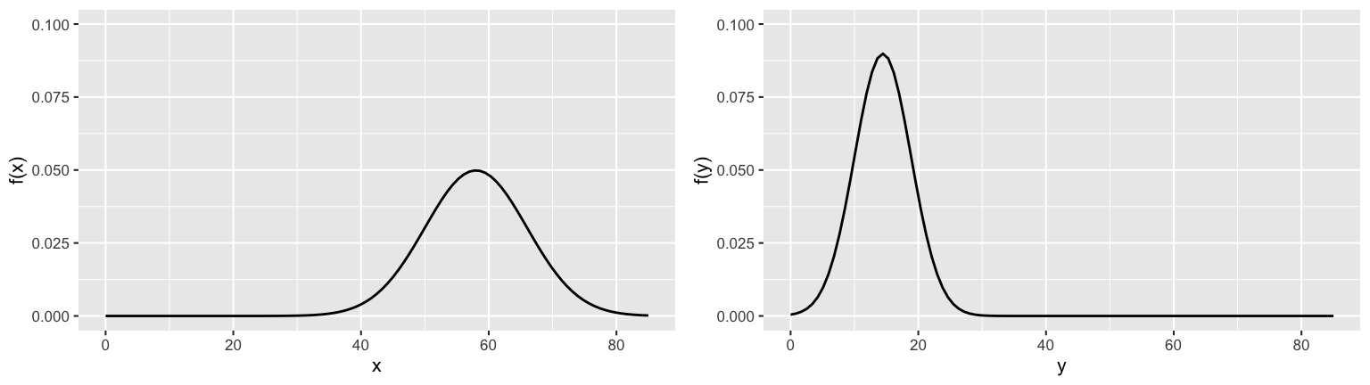
Let \(X\) be the high temperature (F) on an October day in St Paul where \[X \sim N(58, 8^2)\] Let \(Y\) be the high temperature in Celsius, thus \(Y = (X - 32)*5/9\):
Let \(X\) be the number of fair coin flips until we observe Heads. Then \[X \sim Geo(0.5)\] Suppose we win \(Y = X^2\) dollars (eg: $1 for 1 roll, $4 for 2 rolls, $9 for 3 rolls, etc).
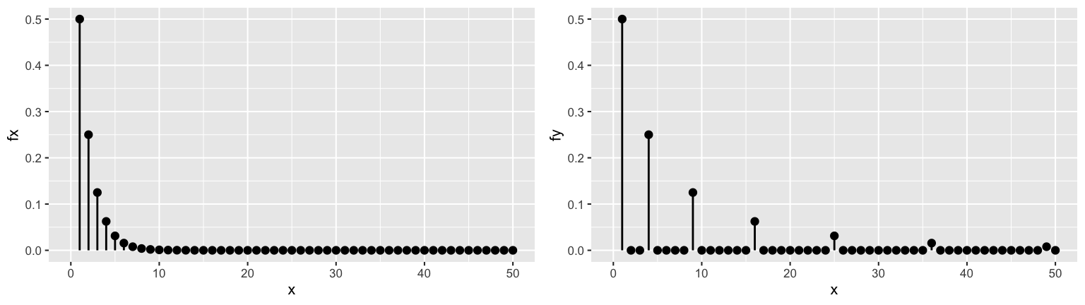
EXAMPLE 1: Functions of discrete RVs
Build the pmf of \(Y\), \(p_Y(y)\), the earnings in our coin flip game.
EXAMPLE 2: Functions of continuous RVs
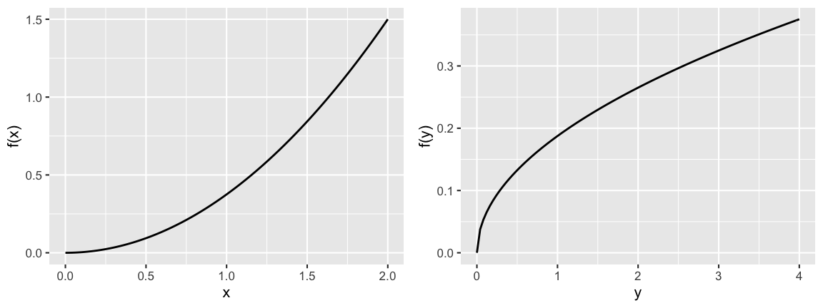
Let continuous RV \(X\) have pdf and cdf \[f_X(x) = 0.375 x^2 \;\; \text{ for } x \in (0,2) \;\;\; \text{ and } \;\;\; F(x) = \begin{cases} 0 & x < 0 \\ 0.125 x^3 & 0 \le x < 2 \\ 1 & x \ge 2 \\ \end{cases}\]
Let \(Y = X^2\) and build the pdf of \(Y\), \(f_Y(y)\). THINK: Why isn’t it \(f_X(\sqrt{y})\)?
14.2 Exercises
In the previous activity, you explored many linear transformations of RV \(X\):
\[Y = aX + b\]
Such transformations are common. For example:
\(X\) = temperature in Fahrenheit
\(Y = \frac{5}{9}(X-32)\) = temperature in Celsius\(X\) = height in centimeters
\(Y = 2.54 X\) = height in inches
We’ll study the properties of linear transformations below.
14.2.1 Part 1: Linear transformation of the Uniform
Consider the specific setting in which \(X \sim \text{Unif}(0,1)\) with
\[\begin{split} f_X(x) & = 1 \;\; \text{ for } x \in [0,1] \\ F_X(t) & = \begin{cases} 0 & t < 0 \\ t & 0 \le t < 1 \\ 1 & t \ge 1 \\ \end{cases} \\ E(X) & = 1/2, \;\; E(X^2) = 1/3, \;\; Var(X) = 1/12 \\ \end{split}\]
Further, let \(Y\) be the following linear transformation of \(X\) where \(d > c\):
\[Y = g(X) = (d-c)X + c\]
Recall that in your simulations, you observed that linear transformations of a Uniform RV are still Uniform, but with different expected value and variance. You’ll now provide mathematical proof!
Expected value of \(Y\)
We know that \(E(X) = 0.5\). What does this tell us about \(E(Y)\)?- Calculate \(E(Y)\) using only the properties of \(f_X\) and the definition of \(E(X)\): \[E(Y) = E((d-c)X + c) = \int_0^1 ((d-c)x + c)f_X(x) dx = \text{???}\] NOTE: Don’t do any new calculus!
- Calculate \((d-c)E(X) + c\). This should equal your answer to part a!
Variance of \(Y\)
Similarly, we know that \(E(X^2) = 1/3\) and \(Var(X) = 1/12\). What about \(E(Y^2)\) and \(Var(Y)\)?Calculate \(E(Y^2)\) using only \(f_X(x)\), \(E(X)\) and \(E(X^2)\): \[\begin{split} E(Y^2) = E(((d-c)X + c)^2) & = E((d-c)^2X^2 + 2c(d-c) X + c^2) \\ & = \int_0^1 ((d-c)^2x^2 + 2c(d-c) x + c^2) f_X(x) dx \\ & = \text{???} \end{split}\]
Again, don’t do any new calculus!- Combine this with your calculation of \(E(Y)\) above to calculate \(Var(Y) = E(Y^2) - [E(Y)]^2\)
Calculate \((d-c)^2 Var(X)\). This should equal your answer to part b!
pdf of \(Y\)
The expected value and variance, \(E(Y)\) and \(Var(Y)\), provide key features of \(Y\). But what can we say about overall model of \(Y\)?- Derive the pdf of \(Y\), \(f_Y(y)\). Hint: First derive \(F_Y()\) from \(F_X()\), then \(f_Y()\) from \(F_Y()\).
- Sketch \(f_Y(y)\).
- This should all look familiar! Specify the model of \(Y\).
- General setting
In the exercise above you proved that a linear transformation of a Uniform is Uniform! You’ll now extend these observations to the general setting in which \(X\) is some RV and \(Y = aX + b\).- Prove \(E(Y) = E(aX + b) = aE(X) + b\) for continuous RVs. The proof for discrete RVs is similar.
- Prove \(Var(Y) = Var(aX + b) = a^2\text{Var}(X)\) for continuous RVs. The proof for discrete RVs is similar. HINT: Starting from the definition \(Var(Y) = E[(X - E(X))^2]\) might be easier!
- For discrete RV \(X\), prove that \[p_Y(y) = p_X\left(\frac{y - b}{a} \right)\]
- For continuous RV \(X\), prove that \[f_Y(y) = \frac{1}{|a|}f_X\left(\frac{y - b}{a} \right)\] HINT: consider 2 unique cases: \(a \ge 0\) and \(a < 0\).
Solution
Assume \(X\) is continuous. The proof for discrete \(X\) is similar.
\[\begin{split} E(Y) & = E(aX + b) \\ & = \int (ax+b)f_X(x)dx \\ & = \int (axf_X(x) + bf_X(x))dx \\ & = a\int xf_X(x)dx + b\int f_X(x)dx \\ & = aE(X) + b \\ & \\ Var(Y) & = Var(aX + b) \\ & = E((aX+b - E(aX+b))^2) \\ & = E((aX - aE(X)))^2) \\ & = E(a^2(X - E(X))^2) \\ & = a^2 E((X - E(X))^2) \;\;\;\; \text{ (we've seen we can take constants out of E()} \\ & = a^2 Var(X) \\ & \\ \text{ when } a > 0: & \\ F_Y(y) & = P(Y \le y) \\ & = P(aX+b \le y) \\ & = P(X \le (y-b)/a) \\ & = F_X((y-b)/a) \\ f_Y(y) & = F'_Y(y) = \frac{1}{a}f_X((y-b)/a) \\ & \\ \text{ when } a < 0: & \\ F_Y(y) & = P(Y \le y) \\ & = P(aX+b \le y) \\ & = P(X \ge (y-b)/a) \\ & = 1 - P(X \le (y-b)/a) \\ & = 1 - F_X((y-b)/a) \\ f_Y(y) & = F'_Y(y) = \frac{1}{-a}f_X((y-b)/a) = \frac{1}{|a|}f_X((y-b)/a) \\ \end{split}\]
14.2.2 Part 2: Linear transformation of the Normal
In Part 2, you’ll examine linear transformations of a Normal RV. Recall that if \(X \sim N(\mu, \sigma^2)\) then
\[f_X(x) = \frac{1}{\sqrt{2\pi}} \exp\left\lbrace -\frac{1}{2}\left(\frac{x - \mu}{\sigma} \right)^2\right\rbrace\]
- Application to the Normal model
Let \(X\) be the high temperature (F) on an October day in St Paul where \[X \sim N(58, 8^2)\] Let \(Y\) be the high temperature in Celsius, thus \(Y = (X - 32)*5/9\).- What are the expected value and variance in October temperatures, in degrees Celsius?
- What is the probability model of \(Y\), \(Y \sim ???\). Provide proof.
- Linear transformations of Normal is Normal
- Consider taking a linear transformation of the standard Normal \(Z \sim N(0,1)\): \[X = \sigma Z + \mu\]
- Prove that \(E(X) = \mu\) and \(Var(X) = \sigma^2\).
- It’s nice to know these features of \(X\), but many models can have these same mean and variance. Better yet, prove that \(X\) is Normal, \[X \sim N(\mu,\sigma^2)\]
Consider taking a linear transformation of \(X \sim N(\mu,\sigma^2)\), \[Z = \frac{X - \mu}{\sigma}\] Construct \(E(Z)\), \(Var(Z)\), and the model of \(Z\).
What’s the significance of these results?!
- Consider taking a linear transformation of the standard Normal \(Z \sim N(0,1)\): \[X = \sigma Z + \mu\]
14.2.3 Part 3: More
- Is a linear transformation of a Binomial itself Binomial? Explain.
Bonus
Let \(X \sim Unif(0,1)\) and \(Y\) be a continuous RV with \[\begin{split} f_Y(y) & = 0.02 y \;\; \text{ for } y \in (0,10) \\ F_Y(y) & = \begin{cases} 0 & y < 0 \\ 0.01 y^2 & 0 \le y < 10 \\ 1 & y \ge 10 \\ \end{cases} \end{split}\]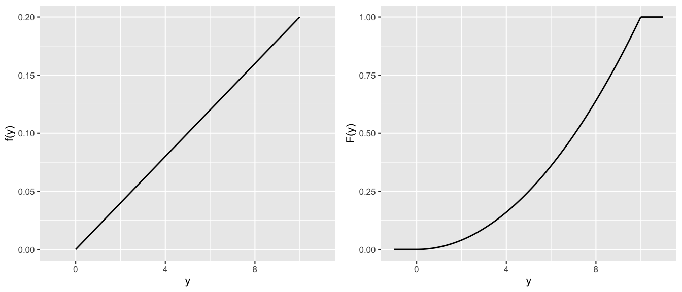
Prove that \(Y\) is the following nonlinear transformation of \(X\):
\[Y = \sqrt{\frac{X}{0.01}}\]
14.3 Summary
Linear Transformations
For RV \(X\) (discrete or continuous), let \[Y = aX + b \;\; \text{ for } a,b \in \mathbb{R}\] Then \[\begin{split} E(Y) & = a E(X) + b \\ Var(Y) & = a^2 Var(X) \\ \end{split}\]
Further,
\[\begin{split}
X \text{ discrete } \Rightarrow \;\; & p_Y(y) = p_X\left(\frac{y - b}{a} \right) \\
X \text{ continuous } \Rightarrow \;\; & f_Y(y) = \frac{1}{|a|}f_X\left(\frac{y - b}{a} \right) \\
\end{split}\]
Interpretation
- \(a\) = a change in scale and \(b\) = a change in location
- The expected value of a RV is impacted by both a change in location (\(b\)) and scale (\(a\))
- The variance of a RV isn’t impacted by a change in location (\(b\)) but is impacted by a change in scale (\(a\)).