Probability models
Binomial (& Bernoulli)
Let discrete RV \(X\) be the number of successes in \(n\) trials where:
- the trials are independent;
- each trial has an equal probability \(p\) of success
Then \(X\) is Binomial with parameters \(n\) and \(p\):
\[X \sim Bin(n,p)\] with pdf \[f(x) = P(X=x) = \left(\begin{array}{c} n \\ x \end{array} \right) p^x (1-p)^{n-x} \;\; \text{ for } x \in \{0,1,2,...,n\}\]
Properties:
\[\begin{split}E(X) & = np \\ Var(X) & = np(1-p) \\ \end{split}\]
NOTE:
In the special case in which \(n=1\), ie. we only observe 1 trial, then \[X \sim Bern(p)\] That is, the \(Bern(p)\) and \(Bin(1,p)\) models are equivalent.
Consider some plots of Binomial RVs for different parameters \(n\) and \(p\):
<img src="354_manual_spring_20_files/figure-html/unnamed-chunk-229-1.png" width="576" style="display: block; margin: auto;" />In R: Suppose \(X \sim Bin(n,p)\)…
# Calculate f(x)
dbinom(x, size=n, prob=p)

# Calculate P(X <= x)
pbinom(x, size=n, prob=p)

# Plot f(x) for x from 0 to n
library(ggplot2)
x <- c(0:n)
binom_data <- data.frame(x=x, fx=dbinom(x, size=n, prob=p))
ggplot(binom_data, aes(x=x, y=fx)) +
    geom_point()
Uniform (discrete)
Suppose discrete RV \(X\) is equally likely to be any value in the discrete set \(S = \{s_1,s_2,...,s_n\}\). Then \(X\) has a discrete uniform distribution on \(S\) with pdf
\[f(x) = P(X=x) = \frac{1}{n} \;\; \text{ for } x \in \{s_1,s_2,...,s_n\}\]
Geometric
Let discrete RV \(X\) be the number of trials until the 1st success where:
- the trials are independent;
- each trial has an equal probability \(p\) of success
Then \(X\) is Geometric with parameter \(p \in (0,1]\):
\[X \sim Geo(p)\]
with pdf \[f(x) = P(X=x) = (1-p)^{x-1}p \;\; \text{ for } x \in \{1,2,...\}\]
Properties:
\[\begin{split} E(X) & = \frac{1}{p} \\ \text{Mode}(X) & = 1 \\ Var(X) & = \frac{1-p}{p^2} \\ \end{split}\]
Notes:
- \(f(x) = (\text{probability of $x-1$ failures}) * (\text{probability of 1 success})\)
- There are other parameterizations of the geometric distribution. They are used in different ways but produce the same “answer”.
Consider some plots of Geometric RVs for different parameters \(p\):
In R: Suppose \(X \sim Geo(p)\)…
# Calculate f(x)
dgeom(x-1, prob = p)

# Calculate P(X <= x)
pgeom(x-1, prob = p)

# Plot f(x) for x from 1 to m (you pick m)
library(ggplot2)
x <- c(1:m)
geo_data <- data.frame(x = x, fx = dgeom(x-1, prob = p))
ggplot(geo_data, aes(x = x, y = fx)) +
    geom_point()
Poisson
Let discrete RV \(X \in \{0,1,2,...\}\) be the number of events in a given time period. The outcome of \(X\) depends upon parameter \(\lambda>0\), the rate at which the events occur (ie. the average number of events per time interval). In this setting, we can often model \(X\) by a Poisson distribution: \[X \sim Pois(\lambda)\] with pdf \[f(x) = P(X=x) = \frac{\lambda^x e^{-\lambda}}{x!} \;\; \text{ for } x \in \{0,1,2,...\}\]
Properties: \[\begin{split}E(X) & = \lambda \\ Var(X) & = \lambda \\ \end{split}\]
Consider some plots of Poisson RVs for different parameters \(\lambda\):

In R: Suppose \(X \sim Pois(a)\)…
Uniform (continuous)
If continuous RV \(X\) is uniformly distributed across the interval \([a,b]\), then
\[X \sim Unif(a,b)\]
with pdf
\[f(x) = \frac{1}{b-a} \;\; \text{ for } x \in [a,b]\]
Properties: \[\begin{split}E(X) & = \frac{a+b}{2} \\ Var(X) & = \frac{(b-a)^2}{12} \\ \end{split}\]
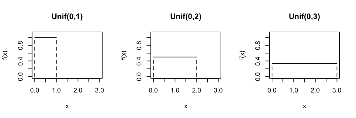
Consider the Uniform distribution for different parameters \(a\) and \(b\):

In R: Suppose \(X \sim Unif(a,b)\)…
# Calculate f(x)
dunif(x, min = a, max = b)

# Calculate P(X <= x)
punif(x, min = a, max = b)

# Plot f(x) for x from a-1 to b+1 (you pick the range)
ggplot(NULL, aes(x = c(a-1, b+1))) +
    stat_function(fun = dunif, args = list(min = a, max = b))
Beta
The Beta distribution can be used to model a continuous RV \(X\) that’s restricted to values in the interval [0,1]. It’s defined by two shape parameters, \(\alpha\) and \(\beta\):
\[X \sim Beta(\alpha,\beta)\]
with pdf
\[f(x) = \frac{\Gamma(\alpha + \beta)}{\Gamma(\alpha)\Gamma(\beta)} x^{\alpha-1} (1-x)^{\beta-1} \;\; \text{ for } x \in [0,1]\]
NOTE: For positive integers \(n\), the gamma function simplifies to \(\Gamma(n) = (n-1)!\). Otherwise, \(\Gamma(z) = \int_0^\infty x^{z-1}e^{-x}dx\).
Properties: \[\begin{split} E(X) & = \frac{\alpha}{\alpha + \beta} \\ Mode(X) & = \frac{\alpha-1}{\alpha+\beta-2} \\ Var(X) & = \frac{\alpha \beta}{(\alpha + \beta)^2(\alpha+\beta+1)}\\ \end{split}\]
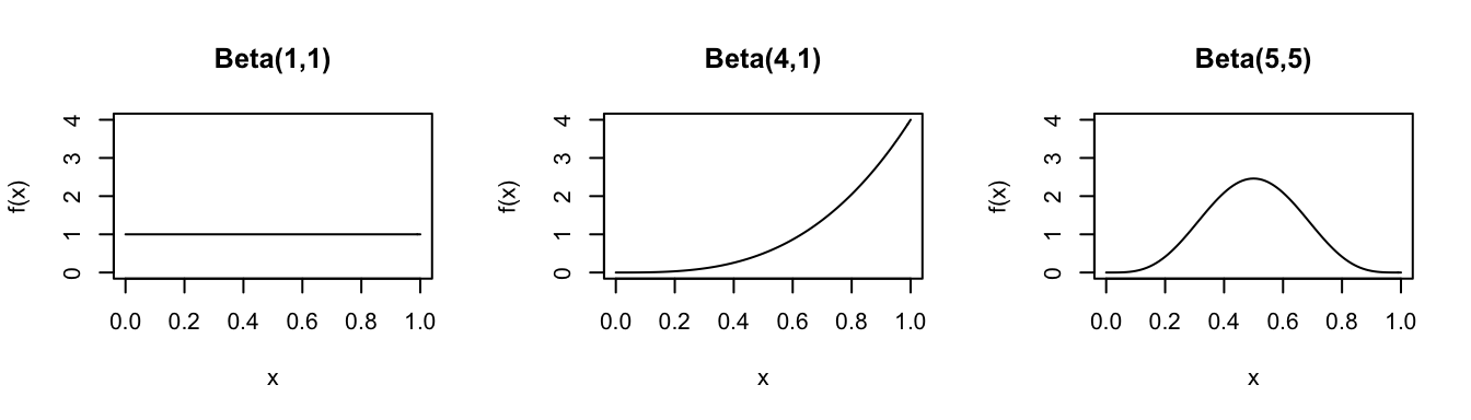
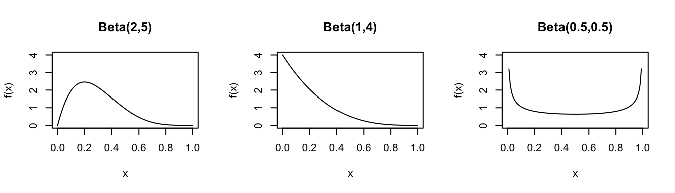
Consider the Beta distribution for different parameters \(\alpha\) and \(\beta\):
In R: Suppose \(X \sim Beta(a,b)\)…
# Calculate f(x)
dbeta(x, shape1 = a, shape2 = b)

# Calculate P(X <= x)
pbeta(x, shape1 = a, shape2 = b)

# Plot f(x) for x from 0 to m (you pick the range)
ggplot(NULL, aes(x = c(0, m))) +
    stat_function(fun = dbeta, args = list(shape1 = a, shape2 = b))
Exponential
Let \(X\) be the waiting time until a given event occurs. For example, \(X\) might be the time until a lightbulb burns out or the time until a bus arrives. The outcome of \(X\) depends upon parameter \(\lambda>0\), the rate at which events occur (ie. the number of events per time period). In this scenario, \(X\) can often be modeled by an Exponential distribution: \[X \sim \text{Exp}(\lambda)\]
with pdf
\[f(x) = \lambda e^{-\lambda x} \;\; \text{ for } x \in [0,\infty)\]
Properties: \[\begin{split} E(X) & = \frac{1}{\lambda} \\ Var(X) & = \frac{1}{\lambda^2} \\ \end{split}\]
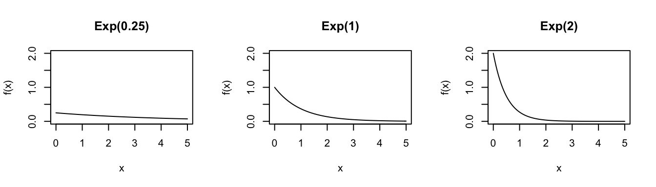
Consider the Exponential distribution for different parameters \(\lambda\):
In R: Suppose \(X \sim Exp(a)\)…
# Calculate f(x)
dexp(x, rate=a)

# Calculate P(X <= x)
pexp(x, rate=a)

# Plot of f(x) for x from 0 to m (you pick the range)
ggplot(NULL, aes(x = c(0, m))) +
    stat_function(fun = dbeta, args = list(shape1 = a, shape2 = b))
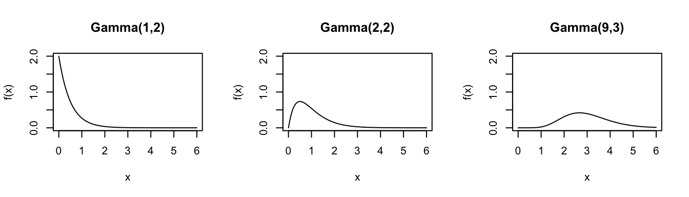
Gamma
The Gamma distribution is often appropriate for modeling positive RVs \(X\) (\(X>0\)) with right skew. For example, let \(X\) be the waiting time until a given event occurs \(s\) times. The outcome of \(X\) depends upon both the shape parameter \(s>0\) (the number of events we’re waiting for) and the rate parameter \(r>0\) (the rate at which the events occur). In this setting, \(X\) can often be modeled by a Gamma distribution: \[X \sim \text{Gamma}(s,r)\]
with pdf \[f(x) = \frac{r^s}{\Gamma(s)}*x^{s-1}e^{-r x} \hspace{.2in} \text{ for } x \in [0,\infty)\] NOTE: For positive integers \(s \in \{1,2,...\}\), the gamma function simplifies to \(\Gamma(s) = (s-1)!\). Otherwise, \(\Gamma(s) = \int_0^\infty x^{s-1}e^{-x}dx\).
Properties: \[\begin{split} E(X) & = \frac{s}{r} \\ Mode(X) & = \frac{s-1}{r} \;\; \text{ (if $s>1$)} \\ Var(X) & = \frac{s}{r^2} \\ \end{split}\]
Consider the Gamma distribution for different parameters \((s,r)\):
In R: Suppose \(X \sim Gamma(s,r)\)…
# Calculate f(x)
dgamma(x, shape = s, rate = r)

# Calculate P(X <= x)
pgamma(x, shape = s, rate = r)

# Plot of f(x) for x from 0 to m (you pick the range)
ggplot(NULL, aes(x = c(0, m))) +
    stat_function(fun = dgamma, args = list(shape = s, rate = f))
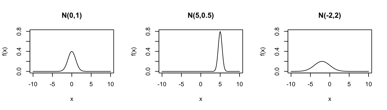
Normal
Let \(X\) be an RV with a bell-shaped distribution centered at \(\mu\) and with variance \(\sigma^2\). Then \(X\) is often well-approximated by a Normal distribution: \[X \sim \text{Normal}(\mu,\sigma^2)\]
with pdf \[f(x) = \frac{1}{\sqrt{2\pi\sigma^2}}*\exp\left\lbrace - \frac{1}{2}\left(\frac{x-\mu}{\sigma} \right)^2 \right\rbrace \hspace{.2in} \text{ for } x \in (-\infty,\infty)\]
Properties: \[\begin{split} E(X) & = \mu \\ Var(X) & = \sigma^2 \\ \end{split}\]
Consider the Normal distribution for different parameters \((\mu,\sigma^2)\):
In R: Suppose \(X \sim N(m,s^2)\)…
# Calculate f(x)
dnorm(x, mean = m, sd = s)

# Calculate P(X <= x)
pnorm(x, mean = m, sd = s)

# Plot f(x) for x from a to b (you pick the range)
ggplot(NULL, aes(x = c(a, b))) +
    stat_function(fun = dnorm, args = list(mean = m, sd = s))