20 Modeling case study

20.1 Discussion

RECALL: THE POISSON MODEL

A Poisson RV $X$ is discrete on $\{0,1,2,...\}$. Typically, the Poisson is used to model $X$, the number of times that an event occurs in a time interval where events are assumed to occur at a rate of $\lambda$ per time interval. In this case, $X$ is often well-approximated by a Poisson model: \[X \sim \text{Pois}(\lambda)\] with \[\begin{split} p_X(x) & = \frac{e^{-\lambda}\lambda^x}{x!} \hspace{.25in} \text{ for } x\in\{0,1,2,...\} \\ M_X(t) & = \exp\left\lbrace \lambda(e^t - 1) \right\rbrace \\ E(X) & = \lambda \\ Var(X) & = \lambda \\ \end{split}\]

Examples

More examples

On average, calls come into a call center at a rate of 4 per minute. Then:

$X$ = number of calls in 1 minute

\[X \sim \text{Pois}(4)\]
$Y$ = number of calls in 30 seconds

\[y \sim \text{Pois}(2)\]
$Z$ = number of calls in 2 minutes

\[z \sim \text{Pois}(8)\]

20.2 Exercises

model	PMF/PDF	$E(X)$	$Var(X)$	$M_X(t)$
Bin($n,p$)	$\left(\begin{array}{c} n \\ x \end{array} \right) p^x (1-p)^{n-x}$	$np$	$np(1-p)$	$(1 - p + pe^t)^n$
Pois($\lambda$)	$\frac{\lambda^x e^{-\lambda}}{x!}$	$\lambda$	$\lambda$	$\exp\left\lbrace \lambda(e^t - 1) \right\rbrace$
Exp($\lambda$)	$\lambda e^{-\lambda x}$	$\frac{1}{\lambda}$	$\frac{1}{\lambda^2}$	$\frac{\lambda}{\lambda - t}$ for $t < \lambda$
N($\mu,\sigma^2$)	$\frac{1}{\sqrt{2\pi\sigma^2}} \exp\left\lbrace -\frac{1}{2}\left(\frac{x-\mu}{\sigma} \right)^2\right\rbrace$	$\mu$	$\sigma^2$	$\exp \left\lbrace \mu t + \frac{1}{2}\sigma^2 t^2\right\rbrace$

Goals

The following case study exercises bring together many recent course concepts. It will be due as homework though you’ll have class time to start it.

The story

Suppose that the average adult female spider lays an average of 100 eggs per month. Suppose that, independently, each egg has a 0.50 probability of surviving/hatching. Let’s randomly select a female spider and monitor her for a month. Let $Y$ = number of eggs laid in a month, and let $X$ = number of eggs that hatch.

Poisson features
Our study of spiders will utilize the Poisson model. Thus, we need to be able to describe features of a Poisson. To this end, consider some RV $X \sim Pois(\lambda)$. Then $X$ has pmf \[p_X(x) = \frac{e^{-\lambda}\lambda^x}{x!} \;\; \text{ for } x \in \{0,1,2,...\}\]
1. Prove that $X$ has mgf $M_X(t)=e^{\lambda(e^t−1)}$.
  HINT: Recall that $M_X(t) = E(e^{tX})$
2. Set up a formula that we could use to calculate $E(X)$ directly from the pmf $p_X(x)$. (You do not need to solve this formula.)
3. Alternatively, use the mgf to prove that \[E(X) = Var(X) = \lambda\]
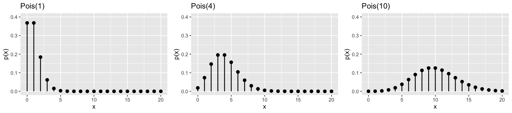
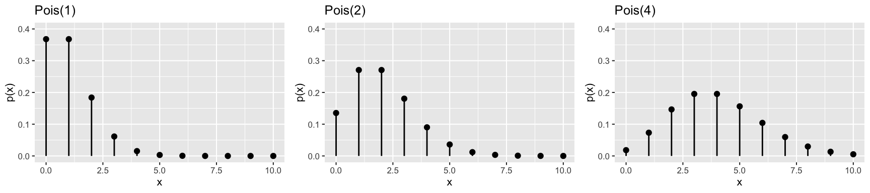
4. Use these results to fill in the table for the Poisson RVs illustrated below:
  
  RV $p_X(x)$ $E(X)$ $Var(X)$
  
  $X \sim Pois(1)$
  
  $X \sim Pois(2)$
  
  $X \sim Pois(4)$

Poisson for spiders
Based on spider research, it’s reasonable to assume that $Y \stackrel{\cdot}{\sim} \text{Pois}(100)$: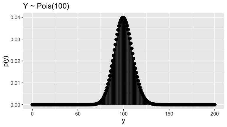

Fill in the following table of features for $Y$.

Feature Result Details

pmf support:

$E(Y)$ units:

$Var(Y)$ units:

Feature	Result	Details
pmf		support:
\(E(Y)\)		units:
\(Var(Y)\)		units:

Poisson & Exponential
(NOTE: You’ve seen a very similar exercise before! This is an important concept, thus important to see again. Try this exercise from scratch before peaking at your earlier work.)

You’ve seen that the Uniform(0,1) is a special case of the Beta, that the Exponential is a special case of the Gamma, and other connections between models. One very satisfying connection is that between the Poisson and Exponential models Again let $Y \sim \text{Pois}(100)$ be the number of bug eggs laid per month where we would typically expect 100 eggs to be laid. Let $W$ be the waiting time (in months) between 2 eggs being laid.
1. Suppose an egg is laid at time “0”. Let $Z$ be the number of eggs that are laid in the next $w$ months, ie. in $(0, w]$. State the model of $Z$ along with its pmf $f_Z(z)$. NOTE: This should depend on $w$.
2. Calculate the probability that 0 eggs are laid in the next $w$ months, $P(Z=0)$. NOTE: This should depend on $w$.
3. Derive a formula for the CDF of $W$, the waiting time for the next egg to be laid: \[F_W(w) = P(W \le w)\] HINT: Rewrite $F_W(w)$ in terms of $P(Z=0)$.
4. Derive the PDF of $W$, $f_W(w)$, and use this to identify the model of $W$. Specify the name of the model and any parameters upon which it depends.

Conditional model of $X$ given $Y=y$
Now that we have a grasp on the number of eggs laid in a month ($Y$), let’s move on to the number of eggs that hatch in a month ($X$). Recall that, independently, each egg has a 0.50 probability of surviving/hatching. Of course, the number of eggs that hatch ($X$) is also limited by the number that are laid ($Y$)!
1. Suppose that a spider lays $Y=y$ eggs in a given month. What’s the conditional model of $X|Y=y$? Name this model and specify any parameters upon which it depends. \[X|(Y=y) \sim ???\] HINT: The conditional model of $X$, hence its parameters, will depend on $y$! You might first assume a specific case (eg: $Y=100$) and generalize your observations to the general case.
2. Write down the conditional PMF $p_{X|Y=y}(x|y)$. Simplify the PMF as much as possible and be sure to specify the support.
3. Use the conditional PMF to fill in the table below. Be sure to show work and use correct notation to indicate how you’re using the PMF.
  
  Quantity Answer
  
  Probability that 10 eggs hatch if 50 are laid.
  
  Probability that 25 eggs hatch if 50 are laid.
  
  Probability that 25 eggs hatch if 30 are laid.
4. Which of the events studied in the above table is the most likely to occur?

Quantity	Answer
Probability that 10 eggs hatch if 50 are laid.
Probability that 25 eggs hatch if 50 are laid.
Probability that 25 eggs hatch if 30 are laid.

Joint model of $X$ and $Y$
Thus far, we have a sense of the conditional variability in the number of eggs that hatch ($X$) given the number that are laid ($Y$), $p_{X|Y=y}(x|y) = P(X=x|Y=y)$. We also have a sense of the marginal variability in the number of eggs that are laid each month ($Y$), $p_Y(y)$. Let’s combine these to model the joint variability in the number of eggs that are laid and hatched.
1. Prove that the joint PMF of $X$ & $Y$ is \[p_{X,Y}(x,y) = \frac{e^{-100}50^y}{x!(y-x)!} \;\; \text{ for } x\in\{0,...,y\}, y\in\{0,1,2,...\}\]
2. Use the joint PMF to fill in the table below. Be sure to show work and use correct notation to indicate how you’re using the PMF.
  
  Quantity Answer
  
  Probability that 10 eggs hatch & 50 are laid.
  
  Probability that 25 eggs hatch & 50 are laid.
  
  Probability that 25 eggs hatch & 30 are laid.

Quantity	Answer
Probability that 10 eggs hatch & 50 are laid.
Probability that 25 eggs hatch & 50 are laid.
Probability that 25 eggs hatch & 30 are laid.

Marginal model of $X$
Above you’ve specified how $X$, the number of eggs that hatch in a month, jointly and conditionally varies with $Y$, the number of eggs that are laid. From this we can construct an understanding of the marginal behavior of egg hatching.
1. Derive the marginal PMF of the number of eggs that hatch in a month, $p_X(x)$. HINTS: \[\begin{split} \sum_{y}p_{X,Y}(x,y) & = \sum_{y=x}^\infty p_{X,Y}(x,y) \;\; \text{ (since $y\ge x$)} \\ e^a & = \sum_{z=0}^\infty \frac{a^z}{z!} \\ \sum_{y=x}^\infty \frac{50^y}{(y-x)!}& = \sum_{z=0}^\infty \frac{50^{z+x}}{z!} \;\;\; \text{ (substituting $z=y-x$)}\\ \end{split}\]
2. This PMF should look familiar! Specify the name of the marginal model of $X$ along with any parameters upon which it depends: \[X \sim ???\]
3. Use the marginal PMF to fill in the table below. Be sure to show work and use correct notation to indicate how you’re using the PMF.
  
  Quantity Answer
  
  Probability that 10 eggs hatch
  
  Probability that 25 eggs hatch

Quantity	Answer
Probability that 10 eggs hatch
Probability that 25 eggs hatch

Conditional model of $Y$ given $X=x$
We’ve derived the conditional model of $X$ given $Y$ - now let’s consider the reverse. That is, suppose we observe that $X=x$ eggs hatched in a month. What does this tell us about the number of eggs that were laid, $Y$? To this end, we’ll derive the conditional PMF of $Y|(X=x)$.
1. Simplifying as much as possible, find a formula for the conditional PMF of $Y$ given $X=x$, $p_{Y|(X=x)}(y|x)$. NOTE: This won’t be a familiar PMF. Further, this conditional PMF and its support will both depend upon $x$.
2. Use the conditional PMF to fill in the table below. Be sure to show work and use correct notation to indicate how you’re using the PMF.
  
  Quantity Answer
  
  Probability that if 10 eggs hatch, 50 were laid.
  
  Probability that if 25 eggs hatch, 50 were laid.
  
  Probability that if 25 eggs hatch, 30 were laid.

Quantity	Answer
Probability that if 10 eggs hatch, 50 were laid.
Probability that if 25 eggs hatch, 50 were laid.
Probability that if 25 eggs hatch, 30 were laid.

Model summary
In the exercises above, you built up an understanding for the marginal, joint, and conditional behaviors of the number of spider eggs that are laid and hatched in a given month. Let’s summarize these observations here.

Use the PMFs you derived above to fill in the table below. Be sure to show work and use correct notation to indicate which PMF you’re using and how you’re using it.

Quantity	Answer
Probability that 50 eggs are laid.
Probability that 25 eggs hatch.
Probability that if 25 eggs hatched, 50 were laid.
Probability that 25 eggs hatch if 50 were laid.
Probability that 25 eggs hatch & 50 were laid.

Construct 2 plots in RStudio & sketch these in your homework (no need to print the plots): (1) a plot of the marginal PMF of $X$; and (2) a plot of the conditional PMF of $X$ if $Y=50$. Be sure that these share the same x-axis and y-axis scales (you might have to play around to find scales that capture the full PMFs). Helpful examples are provided below.

library(ggplot2)

# A barplot of Z ~ Bin(200,0.25)
binom_data <- data.frame(x = 0:200, y = dbinom(c(0:200),size=200,prob=0.25))
ggplot(binom_data, aes(x = x, y = y)) + 
  geom_point() +
  geom_segment(aes(x = x, xend = x, y = 0, yend = y)) + 
  labs(x = "z", y = "p(z)") + 
  lims(x = c(0,200), y = c(0,0.07))

# A barplot of Z ~ Pois(100)
pois_data <- data.frame(x = 0:200, y = dpois(c(0:200),lambda=100))
ggplot(pois_data, aes(x = x, y = y)) + 
  geom_point() + 
  geom_segment(aes(x = x, xend = x, y = 0, yend = y)) + 
  labs(x = "z", y = "p(z)") + 
  lims(x = c(0,200), y = c(0,0.07))

For an audience of spider researchers, compare and contrast the 2 models plotted above. (For example, be sure to speak about $X$ in terms of eggs hatching, not as mathematical notation.)
Prove and explain whether $X$ and $Y$ are independent RVs.

Find & exterminate
You and your roommate have a spider problem. You hire an exterminator that advertises the following: “If $X$ is the proportion of your spiders that we exterminate and $Y$ is the proportion of your spiders that we find, we can promise that $(X,Y)$ is uniformly distributed on $0 < X < Y < 1$”. The promised joint pdf of $X$ and $Y$ is illustrated below: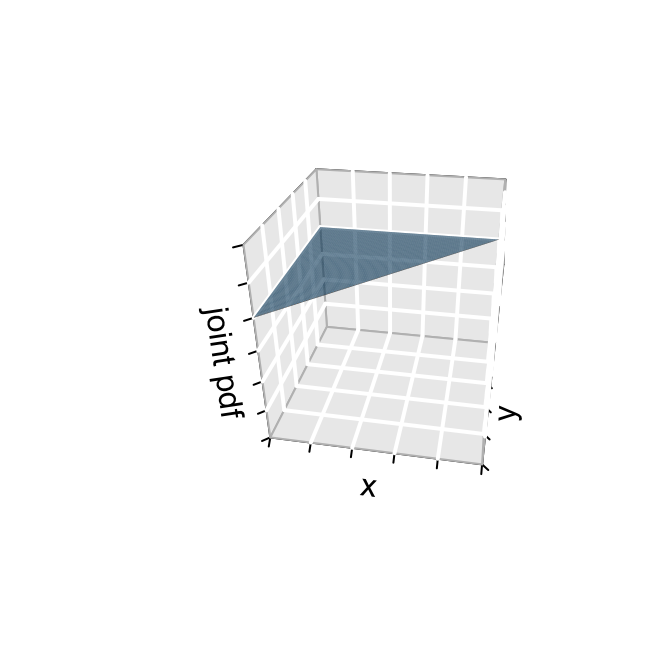

Let’s examine the exterminator’s advertisement.
1. Write out the joint pdf of $X$ and $Y$, $f_{X,Y}(x,y)$. HINT: You can use geometry for this exercise if you wish.
2. Without using geometry, prove that this is a valid pdf. HINT: It would be incorrect to calculate $\int_0^1\int_0^1 f_{X,Y}(x,y)dxdy$.
3. Use the joint pdf to calculate the probability that the exterminator finds less than 50% of the spiders and exterminates less than 25%, $P((X < 0.25) \cap (Y < 0.5))$. ALSO represent this probability in a sketch of the joint pdf.

Marginal model of $Y$
Let’s focus on $Y$, the proportion of spiders that the exterminator finds.
1. Derive the marginal pdf $f_Y(y)$. HINTS: (1) It would be incorrect to calculate $\int_0^1 f_{X,Y}(x,y)dx$; (2) Before doing any calculations, look back at the joint plot to build intuition: what values can $Y$ be? Is it more likely to be close to 0 or close to 1?
2. Sketch AND describe $f_Y(y)$ in context (ie. in a way that tells us about the exterminator).
3. Calculate $P(Y < 0.5)$.

Conditional model of $X$ given $Y=y$
Finally, consider the conditional model of $X$, the proportion exterminated, given $Y$, the proportion found. The plot below might help build intution.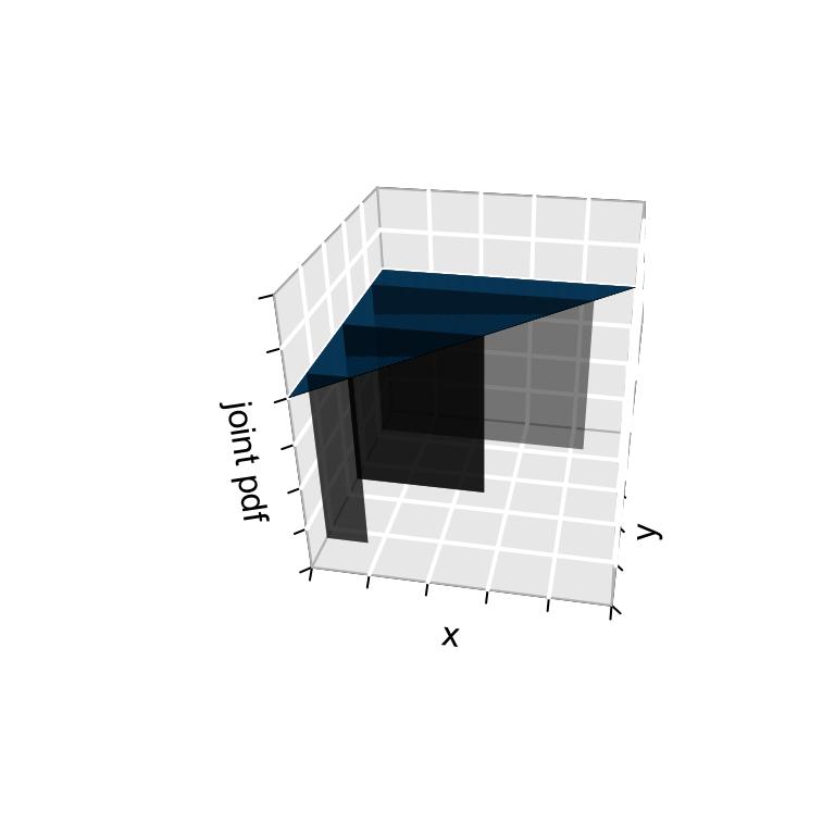
1. Derive the conditional pdf of $X$ when $Y=y$, $f_{X|Y=y}(x|y)$.
2. Prove that this conditional pdf is valid.
3. Consider the specific case in which the exterminator finds 50% of the bugs, $Y = 0.5$. Derive and sketch the conditional pdf of $X$, $f_{X|Y=0.5}(x|y=0.5)$.
4. This PDF should look familiar. Specify the name of this conditional model and any parameters upon which it depends. \[X | (Y = 0.5) \sim ???\]
5. Calculate the conditional probability that if the exterminator finds 50% of the bugs, that less than 25% of the bugs are exterminated, $P(X < 0.25 | Y=0.5)$.
6. Are $X$ and $Y$ independent? Support your answer with mathematical proof.

OPTIONAL: Darts
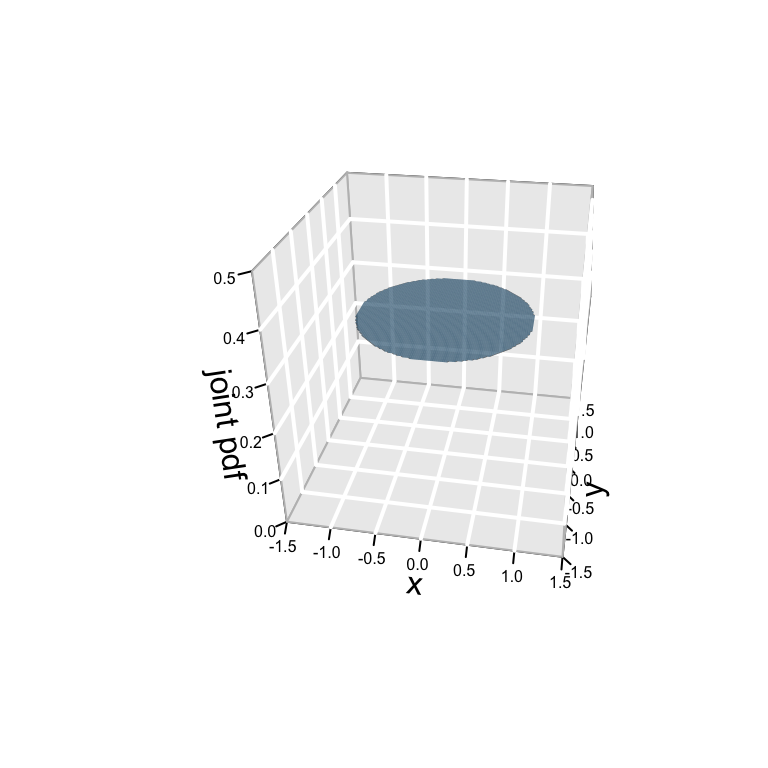
You and your roommate decide to play a game of darts in order to determine who has to clean up the mess. You practice with a dart board that has a radius of 1 foot. You’re a bad dart player, but not that bad. When you throw, you hit the board every time. However, the location of the dart is equally likely to land anywhere on the board. Specifically, if the bullseye is centered at (0,0), your dart location $(X,Y)$ is equally likely to be anywhere on the unit circle: \[X^2 + Y^2 \le 1 \;\] NOTE: $X^2 + Y^2 \le 1$ is equivalent to saying: \[-1 \le X \le 1 \;\; \text{ and } -\sqrt{1-X^2} \le Y \le \sqrt{1-X^2}\] See the plot below.
a. Write out the joint pdf of $X$ and $Y$, $f_{X,Y}(x,y)$. HINTS: (1) Don’t forget that $-1 \le X \le 1$ and $-\sqrt{1-X^2} \le Y \le \sqrt{1-X^2}$; (2) $\int_{-1}^1 \sqrt{1-x^2}dx = \frac{\pi}{2}$; (3) You can use geometry for this exercise if you wish.
b. Without using geometry, prove that this is a valid pdf. HINTS: (1) The following would be incorrect: $\int_0^1\int_0^1 f_{X,Y}(x,y)dydx$.; (2) $\int_{-1}^1 \sqrt{1-x^2}dx = \frac{\pi}{2}$
c. The bullseye area is centered at (0,0) and has a radius of 0.1 feet (1.2 inches). Use the joint pdf to calculate the probability of hitting a bullseye. NOTE: You can use geometry to provide intuition, but your proof must directly utilize the pdf.
d. Derive, sketch, AND describe the marginal pdf $f_X(x)$ of your dart’s $X$-coordinate on the dart board. Be sure that your description is contextually meaningful (ie. talk about darts). NOTE: It would be incorrect to calculate $\int_0^1 f_{X,Y}(x,y)dy$.

OPTIONAL: Blindfolds
Your roommate blindfolds you and tells you to throw a dart. They don’t tell you the exact location, but DO tell you the $X$ coordinate. The following plot might help build intuition: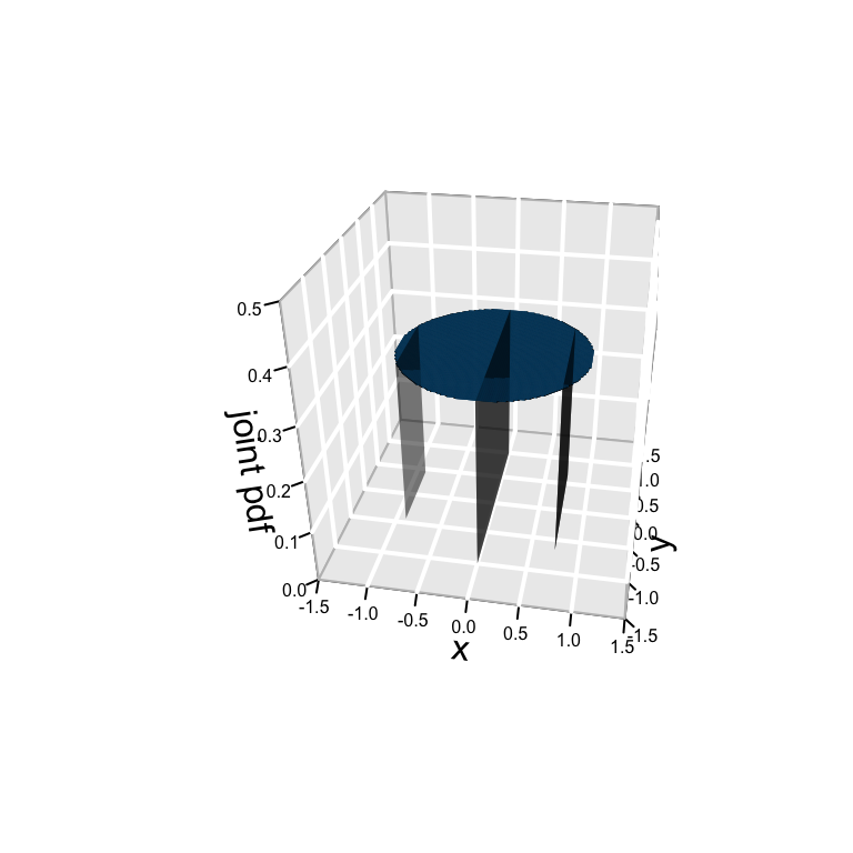
1. Derive the conditional pdf of $Y$ when $X=x$, $f_{Y|X=x}(y|x)$.
2. Prove that this conditional pdf is valid.
3. Suppose your roommate tells you that $X = 0.5$. Derive and sketch the conditional pdf of $Y$, $f_{Y|X=0.5}(y|x=0.5)$.
4. Are $X$ and $Y$ independent? Support your answer with mathematical proof.

model	PMF/PDF	\(E(X)\)	\(Var(X)\)	\(M_X(t)\)
Bin(\(n,p\))	\(\left(\begin{array}{c} n \\ x \end{array} \right) p^x (1-p)^{n-x}\)	\(np\)	\(np(1-p)\)	\((1 - p + pe^t)^n\)
Pois(\(\lambda\))	\(\frac{\lambda^x e^{-\lambda}}{x!}\)	\(\lambda\)	\(\lambda\)	\(\exp\left\lbrace \lambda(e^t - 1) \right\rbrace\)
Exp(\(\lambda\))	\(\lambda e^{-\lambda x}\)	\(\frac{1}{\lambda}\)	\(\frac{1}{\lambda^2}\)	\(\frac{\lambda}{\lambda - t}\) for \(t < \lambda\)
N(\(\mu,\sigma^2\))	\(\frac{1}{\sqrt{2\pi\sigma^2}} \exp\left\lbrace -\frac{1}{2}\left(\frac{x-\mu}{\sigma} \right)^2\right\rbrace\)	\(\mu\)	\(\sigma^2\)	\(\exp \left\lbrace \mu t + \frac{1}{2}\sigma^2 t^2\right\rbrace\)

RV	\(p_X(x)\)	\(E(X)\)	\(Var(X)\)
\(X \sim Pois(1)\)
\(X \sim Pois(2)\)
\(X \sim Pois(4)\)