16 The Gamma Model
GOAL
Learn a new model of the day: the Gamma!
16.1 Discussion
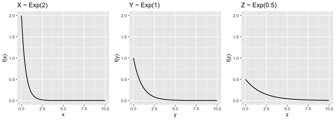
Recall that the exponential model is often used to model a continuous waiting time. Specifically:
\(X > 0\) = the waiting time for the next event to occur
\(\lambda\) = rate at which the event occurs (# of events per time period)
Then \[X \sim \text{Exp}(\lambda)\] with PDF \[f_X(x) = \lambda e^{-\lambda x} \hspace{.25in} \text{ for } x > 0 \; .\]
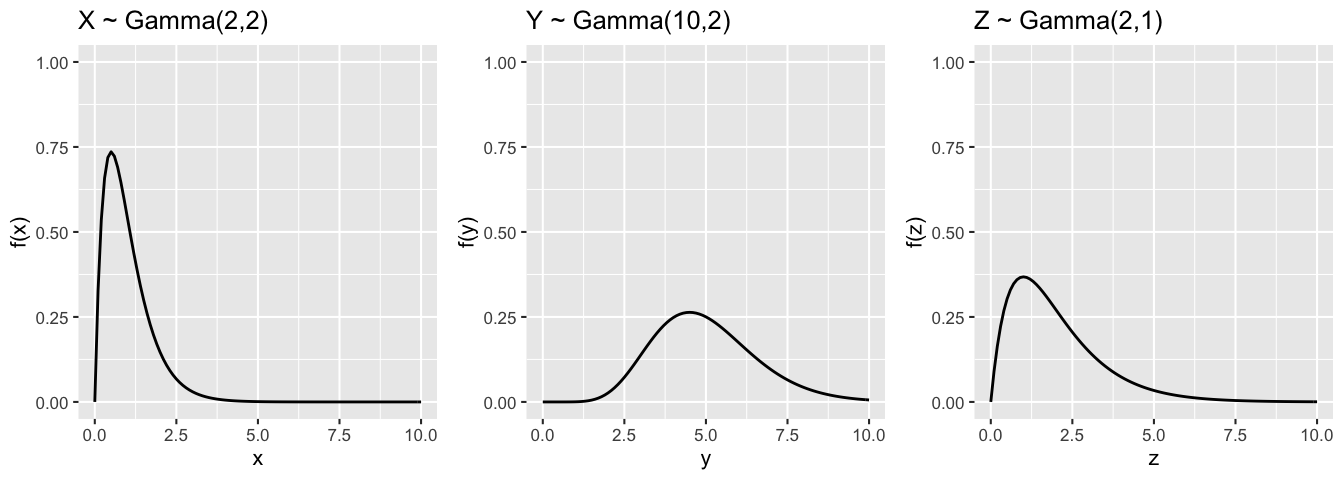
The Gamma model is a generalization of the Exponential. Gamma is often used to model waiting time for multiple events. Specifically:
\(X > 0\) = the waiting time for the event to occur \(a\) times
\(\lambda\) = rate at which the event occurs (# of events per time period)
Then \[X \sim \text{Gamma}(a, \lambda)\] with PDF \[f_X(x) = \frac{\lambda^a}{\Gamma(a)} x^{a-1}e^{-\lambda x} \;\; \text{ for } x>0\] where the “gamma function” \(\Gamma(a)\) has the following properties:
- \(\Gamma(a) = \int_0^\infty x^{a-1}e^{-x}dx\)
- When \(a \in \{1,2,3,...\}\), \(\Gamma(a) = (a-1)!\)
- \(\Gamma(a+1) = a\Gamma(a)\)
GAMMA EXAMPLES
Greg’s selling lemonade on a road where cars pass at a rate of 2 per hour. Sue’s selling lemonade on a road where cars pass at a rate of 1 per hour.
\(X\) = Greg’s waiting time for 2 passing cars: \(X \sim Gamma(2,2)\)
\(Y\) = Greg’s waiting time for 10 passing cars: \(Y \sim Gamma(10,2)\)
\(Z\) = Sue’s waiting time for 2 passing cars: \(Z \sim Gamma(2,1)\)
The trend and variability in these waiting times depend upon \(a\) (the # of events we’re waiting for) and \(\lambda\) (the rate at which these events occur):
16.2 Exercises
Recall that if \(X \sim \text{Gamma}(a, \lambda)\), then
\[f_X(x) = \frac{\lambda^a}{\Gamma(a)} x^{a-1}e^{-\lambda x} \;\; \text{ for } x>0\] where
- \(\Gamma(a) = \int_0^\infty x^{a-1}e^{-x}dx\)
- When \(a \in \{1,2,3,...\}\), \(\Gamma(a) = (a-1)!\)
- \(\Gamma(a+1) = a\Gamma(a)\)
- Exponential vs Gamma
Show that the \(Exp(\lambda)\) RV is a special case of the \(Gamma(a,\lambda)\) RV. HINT: Recall that if \(X \sim Exp(\lambda)\) then \[f_X(x) = \lambda e^{-\lambda x} \;\; \text{ for } x>0\]
- Identify the Gamma
If a RV has a Gamma PDF, then it’s a Gamma RV! Identify the correct model for RVs \(X\) and \(Y\) below.- \(X\) has PDF \(f_X(x) \propto x^9 e^{-2x}\) for \(x > 0\)
- \(Y\) has PDF \(f_Y(y) \propto y^{100} e^{-8y}\) for \(y > 0\)
- \(X\) has PDF \(f_X(x) \propto x^9 e^{-2x}\) for \(x > 0\)
- CHALLENGE: Gamma trend
Derive a formula for the expected waiting time \(E(X)\) for \(a\) events where \(X \sim Gamma(a, \lambda)\). HINTS:- First try to intuit this from the lemonade stories and plots above.
- Then consider using the “make it look like a pdf” summation / integration technique provided below.
- Interpreting Gamma trend
Explain how the Gamma trend is influenced by parameters \(a\) and \(\lambda\).
- Simplifying
Use your previous work to specify a formula for the expected waiting time \(E(X)\) for 1 event where \(X \sim Exp(\lambda)\).
16.3 “Make it look like a pdf” Technique
In many probability calculations, we can utilize the fact that valid PMFs \(p_X(x)\) sum to 1 and valid PDFs \(f_X(x)\) integrate to 1. The main idea:
- Discrete
If we want to calculate \(\sum_x w(x)\) for some function \(w(x)\), we can try to rewrite \(w(x) = c p_X(x)\) for some constant \(c\) and PMF \(p_X(x)\). Then \[\sum_x w(x) = \sum_x c p_X(x) = c \sum_x p_X(x) = c\] - Continuous
If we want to calculate \(\int w(x)dx\) for some function \(w(x)\), we can try to rewrite \(w(x) = c f_X(x)\) for some constant \(c\) and PDF \(f_X(x)\). Then \[\int w(x)dx = \int c f_X(x) dx = c \int f_X(x)dx = c\]